Copyright © W. J. Heitler (2019)
Passive Properties
Note: A listing of the main units and symbols used in equations in this chapter is given here for reference.
The passive properties of a neuron refer to those properties that do not involve voltage-dependent or synaptically activated ion channels. The only ion channels in the membrane are the leakage channels, which have a fixed conductance.
This chapter describes simulations concerning:
- The origin of the resting potential, including the Nernst (equilibrium) potential and the Goldman equation.
- The response of an isopotentialIsopotential means that there is the same membrane potential at every point on the surface. patch of membrane such as a spherical cell or space-clamped axon to a pulse of stimulus current applied across the membrane, including the concepts of time constant and input resistance.
- How passive signals propagate in an axon or dendrite with both delay and attenuation.
Resting potential
All living cells have a potential difference (voltage) across their membranes, usually with the inside negative relative to the outside. In nerve cells the value of the resting membrane potential varies between about -40 mV and -90 mV. This section considers how this is generated.
Note: as well as the simulation activities described in this section, there is an animated tutorial on the origin of the resting potential which, in my opinion (I wrote it), is well worth a visit.
Nernst equation: Equilibrium and reversal potential
A long time ago it was suggested that the resting potential was mainly due to potassium ions (Bernstein, 1902). It was known that potassium ions (K+) have a higher concentration inside the cell than outside, and therefore, if the membrane was permeable to potassium, potassium ions would tend to flow down the concentration gradient and out of the cell. As they left the cell, they would take their positive charge with them. If the cell membrane was only permeable to potassium, then there couldn’t be any accompanying negative ions leaving the cell, and this would leave the inside of the cell negative relative to the outside, which fits with the polarity of the resting membrane potential.
However, the flow would not continue indefinitely. As the inside of the cell became negatively charged it would tend to “pull” the positively-charged K+ ions back into the cell, thus counteracting the concentration gradient. An equilibrium would be achieved if the strength of the negative electrical gradient pulling K+ into the cell exactly balanced the strength of the concentration gradient pushing it out of the cellPerhaps surprisingly, relatively few ions have to cross the membrane to set up this balancing electrical gradient, so the ionic concentration is not significantly altered by the flow.. Essentially, this was Bernstein’s hypothesis to explain the resting potential.
Here is a short video that illustrates the effect:
Dynamic equilibrium at the Nernst potential. Potassium flows down its concentration gradient until the electrical field that develops across the membrane due to the outflow of positive charge is strong enough to repulse potassium and balance the concentration gradient.
At that point equilibrium is achieved, and potassium ions move randomly back and forth across the membrane, with no net flux.
This can be quantified by considering the changes in energy that take place. The change in chemical energy (\(\delta W_c \)) that occurs when particles move down a concentration gradient is: \[ \delta W_c = \delta n.RT.\ln\frac{[X_1]}{[X_2]} \] where \(\delta n\) is the number of particles (ions) that move, R is the gas constant (8.314 J K-1 mol-1), T is the absolute temperature (°K), ln is the natural logarithm (base e), and X1 and X2 are the concentrations on either side of the membrane.
The change in electrical energy (\(\delta W_e \)) that occurs when charged particles move in an electric field is: \[ \delta W_e = \delta n.zFV \] where \(\delta n\) is again the number of particles (ions) that move, z is the charge on each particle (its valency), F is Faraday's number (96485 C mol-1) and V is the strength of the electric field (the membrane potential).
The system will be in equilibrium when the two energies are exactly equal. Rearranging the equations above and cancelling common terms gives the Nernst equation, which for potassium is: \begin{equation} V = \frac{RT}{zF}\ln\frac{[\mathrm{K}_{out}]}{[\mathrm{K}_{in}]} \label{eq:eqNernst} \end{equation} This specifies the membrane potential (\(V\), measured inside relative to outside) which will exactly balance the potassium concentration gradient (\([\mathrm{K}_{out}]/[\mathrm{K}_{in}]\)) . This potential is called the potassium equilibrium potential. If the membrane potential of a cell is equal to the potassium equilibrium potential, potassium will not move into or out of the cell, no matter how permeable the membrane is to potassium.
What happens if the membrane potential is not equalThe difference between the membrane potential and the equilibrium potential of an ion is known as the driving force on that ion, and this will be discussed in detail later. to the equilibrium potential? If it is more positive than the equilibrium potential, potassium will leave the cell because the negative “pull” into the cell is not enough to balance the concentration gradient “push” out of the cell. This will have two effects. First, the loss of positive ions will tend to make the membrane potential more negative, thus moving the potential towards its equilibrium value. Second, the loss of potassium ions will reduce the concentration gradient, thus altering the equilibrium potential itself towards a more positive value. However, the first of these effects normally completely dominates the second. It only takes a relatively small number of ions crossing the membrane to change the potential, and this number is usually only a tiny percentage of the total available, and so it does not normally significantly alter the concentration.
The same argument, but in reverse, applies if the membrane potential is more negative than the equilibrium potential. In this case, potassium moves into the cell, up its concentration gradient, because the electrical “pull” is greater than the concentration ”push”.
Because the direction of ion flow switches as the membrane potential moves on either side of the equilibrium potential, the latter is sometimes also called the reversal potential.
The Nernst equation is general and applies to any ion, not just potassium. If we are dealing with a negative ion such as chloride, the valency (z) becomes negative (or, equivalently, we have to invert the gradient so that it is in/out), but other than that the equation is the same. So all ion types (sodium, potassium, calcium etc.) have their specific equilibrium potential that can be calculated using the Nernst equation, and this potential is dependent on the concentration gradient of that ion across the membrane. Given that the concentrations of different ions vary, it is very likely that different ions will have different equilibrium potentials.
Question: If sodium and calcium had exactly the same concentration gradient across the membrane, would the equilibrium potential be greater for the divalent ion (Ca++) or the monovalent ion (Na+)?
The answer is a bit counter-intuitive, but it makes sense when you remember that it takes more energy to move two charges in an electric field than just one. This means that a half-strength field will balance a given concentration gradient involving a divalent ion compared to the field strength required to balance the same concentration gradient involving a monovalent ion.
We can simplify the rather intimidating full form of equation \eqref{eq:eqNernst} if we roll together the constants, use the more familiar log base 10, assume room temperature (20 °C) and accept an answer in millivolts rather than volts. The equation for potassium then becomes:
\begin{equation} V_{K\:eq\: (mV)} = 58\log_{10}\frac{[K_{out}]}{[K_{in}]}\label{eq:eqSimpleNernst}\end{equation}
The Nernst equation is one of the most important equations in cellular electrophysiology; it underlies the resting potential, the action potential, and synaptic potentials. So it is a good idea to try to understand it.
Take-home message: The Nernst equation specifies a particular trans-membrane voltage, known as the equilibrium potential, that will exactly balance a particular ionic concentration gradient. If the membrane potential is at the equilibrium potential for an ion, there will be no net movement of that ion across the membrane (the current carried by that ion = 0), even if the membrane is highly permeable to the ion.
Potassium Equilibrium Potential
The implications of the Nernst equation can be explored using the Goldman model in Neurosim.
The simulation shows a cell whose membrane is only permeable to potassium. The ion concentrations are approximately those of a mammalian cell. Note that the potassium concentration is a lot higher inside the cell than outside.
The horizontal graph in the upper part of the main Setup view (purple line axis) shows the membrane potential and the potassium equilibrium potential. Because the membrane is only permeable to potassium, these are identical – the Nernst equation \eqref{eq:eqSimpleNernst} applies. The Results view on the right shows the membrane potential as though recorded with a microelectrode. (Note that the “noiseNoise, in this context, means random fluctuations in the signal that carry no useful information.” is purely cosmetic – a real recording would always have some noise in it, but a simulation does not. However, adding it to the simulation emphasises the scrolling nature of the display).
- If the data in the Results view are scrolling too fast for comfort, select a value greater than 0 in the Slow down drop-down list in the main toolbar.
On my computer a value of 10 produces a reasonble scroll rate, but your optimal value may vary. - Hover the mouse over the trace and look at the Status bar at the bottom of the main screen. It should read approximately -90 mV. (If you move the mouse, the read-out changes to reflect the current mouse position.) This matches the potential in the graph in the Setup view.
This resting potential is about right for a glial cell, but it is a bit low for a neuron. We will come back to that later, but for now let’s explore the simple properties.
Temperature Dependence
- Change the temperature to 6°C, and then to 30°C, in turn.
Note that decreasing the temperature causes a depolarization (a decrease in membrane potential), and increasing it causes a hyperpolarization (an increase in membrane potential). This is consistent with the fact that temperature (T) is in the numerator of the full version of the Nernst equation. However, the units in the equation are in absolute temperature, so the effect is relatively small for changes in the biological range.
The direction of change makes intuitive sense since at higher temperatures the ions are more "agitated" (have higher kinetic energy). This means that more ions per second will tend to move across the membrane down their concentration gradient. Hence it takes a stronger barrier (larger membrane potential) to hold them backAt absolute zero the ions wouldn't move at all (they would have no kinetic energy) and you wouldn't need any membrane potential to hold them back!.
- Return the temperature to 20°C.
Concentration Gradient Dependence
Identify the Pause check box at the top of the Results view - you will need to use this soon.
- Increase the extracellular K concentration to 40 mM (simply add a zero to the default value of 4).
- Without waiting, increase the intracellular K concentration to 1400 mM, also by adding a zero.
- Check the Pause box.
Note that the trace jumps up when you made the first change, but then jumps back down to its original value when you made the second change. At this point, the K concentration gradient is the same across the membrane as it was at the start, although the absolute values are 10 times higher.
Take-home message: The equilibrium potential of an ion depends on its concentration gradient across the membrane, but not on the absolute concentration values. This is, of course, implicit in the formula of the Nernst equation \eqref{eq:eqSimpleNernst}.
- Return to the original concentrations (remove the 0s) and uncheck Pause.
- Click the up spin button beside the extracellular K concentration a few times to increase its value in steps of 1, until it reaches a value of 10 mM. Click at about 1 second intervals.
- Click the Pause check box to prevent the data scrolling off the screen while you admire them.
As the extracellular potassium concentration increases, the cell depolarizes. This is because the concentration gradient decreases, so it takes less electrical gradient to balance it. Also note that the step size of the voltage change gets smaller as you repeat the step change in concentration – there is a non-linear voltage response to a linear concentration change.
- Uncheck Pause.
- Set the extracellular concentration to 140 mM. Note that this is the same as the intracellular potassium concentration, and that the membrane potential is zero. With no concentration gradient, no membrane potential is needed to balance it, which makes sense.
- Set the extracellular concentration to 14 mM.
Question: Note that the extracelluar potassium concentration is now one tenth of the intracellular concentration. Look at the value of the membrane potential and at the simplified Nernst equation \eqref{eq:eqSimpleNernst}. You should notice something similar. Can you explain this in terms of the equation?
- Return to the 4 : 140 concentration gradient (you could just reload the file).
- Check the Pause box in the Results view.
- Double the extracellular potassium concentration to 8 mM.
- Uncheck the Pause box and allow the simulation to run just long enough to get a read-out of the new potentials.
- Check the Pause box again.
- Repeat for concentrations of 16, 32, 64, 128 and 256 mM, leaving the display Paused. Make sure that the read-out of the original 4 mM concentration is still visible.
At this point you should have a series of step increases in potential visible in the Results view. Note that the voltage changes are now approximately equal, so there is a linear voltage response to a non-linear concentration change. (In fact, the concentration change is logarithmic, since you are doubling the concentration at each step)
Task: Investigate the relationship between the membrane potential and the extracellular potassium concentration.
-
- Measure the membrane potential at each concentation.
- Check the Measure box at the top of the Results view to open the Measure dialog.
- The dialog is non-modal, so can be kept open while you do experiments.
- Move the dialog so that it does not obscure the Results view.
- Drag the red cursor in the Results view to the X-location for the lowest concentration.
- You can fine-position the cursor with the < and > buttons in the dialog, or the keyboard arrow keys.
- Click the Measure button in the dialog. Note that the data value of each trace appears in the dialog in the labelled columns.
- Repeat the measurements, moving the cursor to the right to the different X-locations appropriate for each concentration .
You should end up with 7 rows visible in the Measure dialog.
Note that at the highest concentration, the membrane potential becomes positive. This is because the concentration gradient has reversed and is now driving K+into the cell, so it takes a positive potential to “repel” the ions and achieve a balance.
- Generate a user column in the Measurement dialog and enter the concentration values.
- Click the +User button to add a column at the left of the measurements.
- Click the column header to edit its label to read [K]ext.
- Click each cell in the user column and enter the concentration.
- You can also navigate between rows with the up and down keyboard arrow keys.
- Plot the voltage against the logarithm (base 10) of the concentration.
- Click the Plot button in the Measure dialog to open the XY Scatter dialog.
- The X axis drop down list should show the text you entered as for the user column header ([K]ext). This is what you want, so leave it alone.
- Select Mem pot (mV) from the Y axis drop down list.
- You should now see a curved line in the plot.
- Check the Log X box.
- Make sure that the base 10 option is selected below the log box, not base e.
- Click the Plot button in the Measure dialog to open the XY Scatter dialog.
- Measure the membrane potential at each concentation.
If you do this correctly, you should end up with a series of points on a straight line.
- Check the Linear trendline box near the bottom of the XY Scatter dialog.
- Note the Slope of the trendline that appears under the checkbox.
Question: How (and why) does the slope relate to the simplified NernstYou may be concerned that the Nernst equation involves a concentration gradient across the membrane, while you are using the value on just one side. However, with the value on the other side fixed, the slope of the plot will be the same in the two cases, although the intercept will differ. equation \eqref{eq:eqSimpleNernst}?
Goldman equation
The Nernst equation \eqref{eq:eqNernst} tells us the equilibrium potential for an ion species with a particular trans-membrane concentration profile. If the membrane is only permeable to that species, then the membrane potential will be equal to the Nernst potential for that species. This is the case with glial cells, where potassium is effectively the only permeant ion. However, neurons, even in the resting state, are usually permeable to more than one ion. What happens then?
Intuitively, it seems likely that the membrane potential will be some sort of weighted compromise between the equilibrium potentials of the various different ions to which the membrane is permeable. Thus if the membrane is mainly permeable to potassium but a little bit permeable to sodium (which is actually the case in a resting neuron), the membrane potential will be close to the potassium equilibrium potential, but pulled a little bit towards the sodium equilibrium potential.
This intuition is formalized in the Goldman-Hodgkin-Katz constant field equation, usually known as the Goldman equation for short (lucky Goldman!). This was derived by considering ion diffusion rates within the membrane in a constant electrical field, which is quite complicated, but the end result is not too bad if you break it down into its bits:
\begin{equation} V = \frac{RT}{F}\ln \left( \frac {P_{\mathrm{K}}[\mathrm{K}_{out}]+P_{\mathrm{Na}}[\mathrm{Na}_{out}]+P_{\mathrm{Cl}}[\mathrm{Cl}_{in}]} {P_{\mathrm{K}}[\mathrm{K}_{in}]+P_{\mathrm{Na}}[\mathrm{Na}_{in}]+P_{\mathrm{Cl}}[\mathrm{Cl}_{out}]} \right) \label{eq:eqGoldman} \end{equation}
The similarity to the Nernst equation is fairly obvious (but note the inversion of the Cl gradient to take account of the negative charge), and most of the symbols have the same meaning. The big difference is that there are 3 ions involved (Na, K and ClThere is an equivalent equation which includes divalent ions like calcium, but this is much more complicated. And since calcium permeability in the resting membrane is very low, we can ignore it in most cases.), and each ion concentration is weighted by the factor Pion, which is the permeability of that ion through the membrane. So clearly, the bigger the permeability, the more influence the ion will have on the Nernst-like equation result.
If we ignore chloride ions the equation can be written in a simpler form:
\begin{equation} V = 58\log \left( \frac {[\mathrm{K}_{out}]+\alpha [\mathrm{Na}_{out}]} {[\mathrm{K}_{in}]+\alpha [\mathrm{Na}_{in}]} \right) \label{eq:eqSimpleGoldman} \end{equation}
Here, the new variable alpha (\(\alpha\)) is the relative membrane permeability of sodium to potassium. Typically, in a resting neuron the potassium permeability is about 25 times greater than the sodium permeability, so \(\alpha\) = 0.04.
Simple Goldman
- Load file Simple Goldman.
- This simulates a cell with a membrane which is permeable to sodium and potassium, and nothing else. It thus implements the simple form of the Goldman equation described above.
In the Setup view the sodium : potassium permeability ratio is shown to the right of the slider bar with a value of 0.04, (and the percentage values to the right of the cell image are 100 and 4 for potassium and sodium respectively). This reflects typical values for a nerve cell.
In the Setup graph (near the top of the screen) note that the membrane potential of -67 mV is depolarized relative to the potassium equilibrium potential (Keq) of -90 mV, but is much closer to that value than it is to the sodium equilibrium potential (Naeq) of +67 mV. The same is seen in the Results view. This reflects the “weighted compromise” mentioned earlier, with the weighting being 100 : 4.
Concentration Dependence
- As previously, increase the extracellular K concentration to 40 mM (simply add a zero to the default value of 4).
- Without waiting, increase the intracellular K concentration to 1400 mM, also by adding a zero.
- Check the Pause box.
Note that the trace jumps up when you made the first change, but then jumps back down when you made the second change. However, unlike with the Nernst equation tutorial, the final potential value is lower than the original, even though the K gradient across the membrane is unchanged.
Take-home message: The membrane potential calculated using the Goldman equation is affected by absolute concentration values, as well as the gradient of values. The higher the overall concentration of an ion, the more it dominates the Goldman equation output.
- Return the K concentrations to their original values.
- Uncheck the Pause box.
Alpha Dependence
There is a slider under the graph in the Setup view which allows you to rapidly adjust the value of alpha (the permeability of sodium relative to potassium).
- Drag the Setup view slider all the way to the right, then all the way to the left, then back towards the middle.
- Click Pause in the Results view.
You should see the membrane potential swing between the sodium and the potassium equilibrium potentials. In fact, by adjusting alpha appropriately, you can “dial up” any membrane potential you like between these two extremes.
Sneak preview: as I expect you know, nerve action potentials (spikes) result from a brief increase in sodium permeability followed by an increase in potassium permeability before returning to the resting state. Thus the membrane potential changes seen in the Results view are a (very crude) reflection of what happens in a spike.
Full Goldman
- Select the Model: Reset command to return to a simulation of the full Goldman equation (this is what you would see if you just ran Goldman from the start).
Note that the resting potential is now -71 mV, which is slightly hyperpolarized compared to previously. This reflects the chloride ions, with their equilibrium potential of -84 mV, adding their “weight” to the compromise.
- Increase the extracellular potassium ion concentrations in steps of 4, 8, 16, 32, 64 and 128 mM. Full details of how to do this were given earlier in the Nernst simulation.
You may notice that the voltage changes occur in unequal step sizes, in contrast to the pure potassium experiment done previously
- Return to the starting potassium concentration (4 mM).
- Increase the relative sodium permeability to 20% (either set the percentage box to 20, or the relative permeability box to 0.2).
- Repeat the changes in potassium concentration as above. The difference in voltage step sizes is now quite marked.
- Measure the membrane potential of this second series at each concentration step as described previously.
Task: Plot the membrane potential voltage against the logarithm (base 10) of the extracellular potassium concentration as described previously. Note that the relationship is now markedly non-linear. However, if you plot the potassium equilibrium potential against the log of the potassium concentration, the relationship is still linear, as indeed it should be from the Nernst equation \eqref{eq:eqNernst}.
Take-home message: If the log plot of concentration against voltage yields a linear relationship, it means that the membrane is only permeable to the ion whose concentration you changed. If plot is non-linear it means that the membrane is also permeable to other ions, and the more non-linear it is, the greater the relative permeability of those other ions.
This was one of the classic experiments that showed that the membrane was predominantly permeable to sodium at the peak of the action potential. You may have already encountered this if you did the walk-through preparing a student activity described elsewhere.
Chloride
Most synaptic inhibition involves opening ion channels that are selectively permeable to chloride ions (as mediated by GABA and glycine ionotropic receptors).
- Use Model: Reset to return to the default conditions.
- Increase the relative permeability of chloride by a factor of 10, from 45% to 450% (just add a 0 to the number).
Note the sudden drop in membrane potential as the chloride permeability increase strengthens the “pull” towards the chloride equilibrium potential, which is negative to the normal resting potential.
Hyperpolarization like this is often part of the mechanism underlying synaptic inhibition. However, the increase in conductance itself has an inhibitory effect due to what is called “shunting”, and this can work even if the chloride equilibrium potential is above resting potential, so that an increase in chloride permeability actually causes depolarization. This is explored further in the Synapse section of the tutorial on depolarizing and silent IPSP.
Developing neurons, and some specialized olfactory neurons, have a very high intracellular chloride concentration (e.g. sensory neurons in the vomeronasal olfactory region; Kim et al., 2015). This can elevate the chloride equilibrium potential considerably.
- Load file Olfactory Chloride.
- This sets the chloride concentration to those measured by Kim et al. The resting relative chloride permeability has been reduced to bring the membrane potential into the correct range of about -50 mV. (This is a guess – it may be that the sodium and potassium values should be changed, but no data are available for these.)
- Increase the chloride permeability by a factor of 10 (just add a 0 to the number).
Now the increased chloride permeability depolarizes the neuron. This would have a strong excitatory effect. In fact, in developing neurons, activation of “inhibitory” chloride channels can actually cause spikes, which may have an important signalling function in developing tissue.
Chloride Regulation
Many cells regulate intracellular chloride concentration; they maintain its valueIn many cell types the chloride equilibrium potential is more depolarized than the resting potential, implying the presence of 'chloride loaders' increasing [Cl-]i above its equilibrium value. However, in some cells, including mature cortical neurons, [Cl-]i is lower than its equilibrium value, and the chloride equilibrium potential is below (more negative than) resting potential. The chloride extrusion is performed by an electroneutral K+-Cl- co-transporter. within a narrow range using pumps and other metabolic mechanisms. The standard Goldman equation assumes that this is the case. However, some cells do not regulate chloride.
- Select Model: Reset.
- Select Passive for the chloride distribution in the Relative Permeability section of the Setup view.
Note that the cell membrane still has the same chloride permeability, but that the intracellular concentration is set as read-only. This is because the intracellular concentration is now determined by the membrane potential, which itself is set only by the potassium and sodium ions (like the Simple Goldman earlier). Chloride will flow into or out of the cell until the chloride gradient across the membrane is in equilibrium with the membrane potential, as determined by the Nernst equation. The extracellular chloride concentration is assumed to be fixed (because the extracellular volume is very large compared to the intracellular volume), so when chloride flows across the membrane, the intracellular but not the extracellular concentration will change. So in this case, rather than the concentration gradients determining the membrane potential, the membrane potential determines the concentration gradient.
- Move the permeability ratio slider to either side, and note that the membrane potential changes as previously. However, also note that the chloride equilibrium potential always equals the membrane potential, and that the intracellular chloride concentration changes while the extracellular concentration remains constant.
IMPORTANT POINT: In the simulation, the intracellular concentration adjusts instantly. However, in a real cell this would take time, maybe considerable time, because to adjust the intracellular concentration a large number of chloride ions might have to flow through a limited number of channels. So in the short term, even if chloride is unregulated, the system will behave as thought the intracellular chloride concentration was fixed, i.e. regulated.
Pumps: Steady State versus Equilibrium
- Select Model: Reset to return to the default starting conditions.
A very important point about the Goldman equation compared to the Nernst equation is that the former describes a steady-state situation, while the latter describes an equilibrium situation. In a typical neuron the membrane potential is not equal to the equilibrium (Nernst) potential of any of the ions, and thus none of the ions are in equilibrium. There is a constant flux of sodium into the cell and potassium out of the cell. [Question: In what direction does chloride move in this scenario?]
The flux of these ions balance each other so that there is no net change in charge across the membrane, and thus no immediate change in membrane potential (if the flux did not balance, the membrane potential would changeDo a thought experiment by considering which ion fluxes would increase and which decrease if the membrane potential changed, and what effect the changed flux would have on the potential. until it did).
On its own this flux would eventually cause the concentration gradients to “run down”, and the cell to depolarize and die. However, there are molecular pumps which push the ions back across the membrane against their concentration gradients, thus keeping the intracellular concentrations in the correct physiological range. The pumps require metabolic energy in the form of ATP to drive them, and form part of the active transport system.
Electrogenic Pumps
The most important pump is the sodium-potassium exchange pump (Na/K ATPase). This pump is electrogenic – it pumps 3 sodium ions out of the cell for every 2 potassium ions that it pumps in. This means that it acts a bit like a battery, and contributes somewhat to the membrane potential of most cells. This contribution is NOT included in any of the simulations so far – they just model the Goldman equation itself, which does not include any pumps at all.
In most neurons the electrogenic Na/K pump makes only a minor direct contribution to the steady-state resting potential, perhaps 5-6 mV, although in some specialised neurons the contribution may be larger (e.g. the olfactory receptor neurons in frogs; Trotier & Døving, 1996). However, the hyperpolarizing effect of the pump can be considerably enhanced if the intracellular sodium concentration ([Na+]i) increases, as can happen after an intense bout of spiking. This is because the pump rate is mainlyIt is also controlled by the extracellular potassium concentration, but if the extracellular volume is relatively large, this does not change very much. controlled by [Na+]i. If the concentration is elevated, the pump rate increases and it makes an enhanced contribution to the membrane potential. It may even hyperpolarize the membrane to a level more negative than the potassium equilibrium potential, which is impossible under standard Goldman conditions. However, this effect is transient - as the sodium is pumped out and its concentration returns to its normal resting level, the pump rate also returns to its normal steady-state level and the extra hyperpolarizing effect disappears.
Permeability vs Conductance
Finally, note that permeability as used in the Goldman equation is not the same as conductance, although the two are closely related. Permeability refers to how easy it is for an ion to cross the membrane, and is largely independent of ion concentration. Conductance refers to how many ions per second (how much current) will flow for a given transmembrane driving forceThe driving force on an ion can be quantified as the difference between the membrane potential and the equilibrium potential of the ion., and is definitely dependent on concentration. This makes sense because if the concentration is very low then there won’t be many ions around, so the flow per second (current) will be low, no matter how easily the individual ions can cross the membrane.
Conductance Asymmetry: Rectification
Given that ion channel conductance can depend on the concentration of the carrier ion, what happens if the concentration is high on one side of the membrane but low on the other? The answer is that the conductance in the high-to-low direction may be higher than in low-to-high concentration direction; a condition known as rectification. For ions like sodium, potassium, and chloride, the physiological concentration range is normally sufficiently high on both sides of the membrane that any difference in conductance is trivial and can be ignored. Such channels are called Ohmic channels, because their conductance is assumed to follow Ohms's Law, in which the conductance is independent of concentration (Ohms's Law is discussed more fully under Basic RC Properties in the next section). The vast majority of publised neural simulations make this assumption, as do most of the simulations in the Neurosim tutorials. However, if the ion concentration is very low indeed on one side of the membrane, rectification can be significant. This is particularly the case for calcium channels, since the free intracellular calcium concentration can indeed be very low. In these cases the current through the membrane can be calculated more accurately using the Goldman-Hodgkin-Katz current equation (note that equation \eqref{eq:eqGoldman} seen previously is the GHK voltage equation), which takes into account membrane potential, permeability and concentration. This is explored further in the Advanced Kinetics section in a later tutorial.
Spherical Cells: The Membrane as a Resistor-Capacitor (RC) Circuit
This section deals with how a simple spherical cell with a passive membrane responds to a stimulus current.
The phospholipid bilayer component of the cell membrane is essentially impermeable to ions, because charged particles cannot easily pass through the hydrophobic central region. This makes the membrane itself an electrical insulator. The electrolyte solutions of the intracellular and extracellular fluid, on the other hand, are electrical conductors. In physics terms, this makes the membrane and its surrounding fluid a capacitor, since the functional definition of a capacitor is two conductors separated by an insulator.
Cell membranes typically contain protein channels (leakage, voltage-dependent and/or synaptic) that allow specific ions to pass through them. These ion channels thus form conductors across the memrane, or, equivalently, resistors but with relatively low resistance. Together, the ion channels and membrane thus form a parallel resistor-capacitor (RCIt would actually be more sensible to call it a conductor-capacitor circuit, since the point of the ion channels that comprise the resistor component is that they are low resistance compared to the phospholipid, which is high resistance. However, we are stuck with the terminology from physics and electronics.) circuit.
In diagrammatic form a patch of membrane can be represented thus:
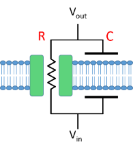
One of the key features of a parallel RC circuit is that the voltage across the resistor is exactly the same as the voltage across the capacitor, because they are linked by low resistance paths (the horizontal wires in the circuit diagram). For a cell, the highly-conductive intra- and extracellular fluids are the functional equivalent of these wires.
A spherical cell of biological proportions can be regarded as an extended patch of such a membrane, wrapped around into a spherical shape. Such a cell would be isopotential – it has the same membrane potential at every point on its surface.
Basic RC Properties
What happens if you record from a spherical neuron with only passive properties, and inject a square pulse of current as a stimulus?
- Load file Passive Cell Body.
- Click the Passive check box in the Setup view to call up the Passive Properties dialog box.
- Click Start.
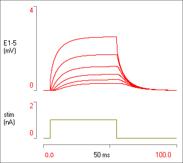
The green trace in the middle is the stimulus, the red trace at the top is the voltage response. Ignore the bottom traces for the moment.
The stimulus has a square waveform, but the voltage response climbs with a rising curve, and then remains at a steady value until the pulse ends, when it falls in a curve symmetrically opposite to the rise. Why does the response have this shape?
When current is injected into the cell it has to go somewhere; it can’t just vanish. It can either charge the capacitor, or flow through the conductor and out of the cell, or a combination of these.
Initially, all the current will go into the capacitor. This is because the capacitor starts off with the resting potential voltage across it, and until there is a change in charge in the capacitor, its voltage cannot change. So the capacitor “holds” the resistor at the resting potential (because they are in parallel). Current flow through a resistor is governed by Ohms law:
\begin{equation} V =IR \label{eq:eqOhmsLaw} \end{equation}where V is voltage, I is current and R is resistance (equivalent to 1/conductance). So if there is no change in the voltage across the resistor (held by the capacitor at its starting value), then there can be no change in current flow through the resistor. Thus all the new applied current goes into the capacitor.
What happens then?
As soon as charge starts to flow into the capacitor, its voltage starts to change according to the following equationThe equation follows from the definition of capacitance: Q = CV, so dQ/dt = C dV/dt.
The rate of flow of charge (dQ/dt) is current, so I = C dV/dt.:
where dV/dt is the rate of change of voltage and C is the capacitance. This means that if we put constant current into a capacitor, there will be a constantly-rising voltage across it. The rate of that rise for a given current depends on the capacitance (bigger capacitors take more charge to change their voltage). If you find this confusing, a bucket analogyIf you pour water (charge) into a bucket (capacitor), the rate at which the water level (voltage) rises depends on how fast you pour in the water (the current), and how wide the bucket (capacitor) is. may help.
HOWEVER, as soon as the voltage across the capacitor starts to rise, the voltage across the resistor also starts to rise because they are in parallel. Now there is a voltage driving some of the current through the resistor. This diverts some of the current that was going into the capacitor into passing through the resistor instead. This means that less current is going into the capacitor and so the rate of voltage change starts to decrease.
Now look at the Neurosim Results view. The red trace shows an initial rapid rate of voltage increase reflecting the high proportion of current going into the capacitor, and then the rate of voltage change drops off as more and more current is diverted through the resistor. Eventually, the voltage rises to a point where all the current goes through the resistor (the capacitor is “fully charged”). At this point there is no more current going into the capacitor, and the voltage no longer changes. The red line has flattened out at its peak value.
Leakage and Capacitive Currents
Now look at the bottom trace. The orange line (only visible in the middle part due to overlay by the cyan trace) shows the current flow through the leakage channels, which is the resistor current in the RC circuit. It exactly parallels the voltage change, thus following the Ohm’s law equation \eqref{eq:eqOhmsLaw}. The cyan line is the total current, including the stimulus. In the middle part the line is at 0 because all the charge coming into the cell from the stimulus is flowing out of the cell through the resistor, leaving a net current of 0. The early downward spike represents the current flow into the capacitor as the membrane depolarizes at the start of the stimulus, and this is not balanced by outward flow through the resistor. The later upward spike represents the current flow out of the capacitor as the membrane repolarizes after the stimulus terminates.
Take-home message: There are two important features in the voltage response of an RC circuit to a constant current:
-
- If you wait long enough, the voltage stabilizes at some final steady-state level.
- The voltage does not get to its final level instantly, but rather rises (and falls) at a curving rate.
These two features can be quantified by the input resistance and the membrane time constant, as described next.
Input Resistance
When the voltage trace has flattened off during the stimulus it means that all the current is passing through the resistor, and hence the capacitor current is 0 (if the capacitor current were non-zero, the voltage would change). We can thus measure the input resistance of the cell. The input resistance is the combined resistance of the total surface membrane of the cell, and is one of the key parameters associated with passive properties. It is a numerical value that gives us a lot of information about how the cell responds to a current stimulus, both in terms of experimental stimuli as in this simulation, and natural stimuli like synaptic currents.
First we want to measure the steady-state voltage change produced by the stimulus.
- Click the Measure check box in the Results view to show the Measure dialog.
- Move the dialog so that it does not obscure the Results view.
- Click the 2 cursors check box in the dialog.
- Note that a red and a blue cursor are now visible in the Results view.
- Drag the red cursor to the flat part of the voltage trace towards the end of the stimulus (about time 48 ms). This is the peak membrane potential achieved during the stimulus.
- Drag the blue cursor to the flat part of the voltage trace before the stimulus starts (the resting potential).
- Click the Measure button in the dialog.
Three rows of data become visible in the dialog. The first (1 red in the Measure Sweep column) shows measurements from the red cursor, the second (1 blue) shows measurements from the blue cursor, and the third (1 red-blue) shows the difference. [If you checked the Only difference box in the dialog, only the third row would show.]
In a purely passive cell the resting potential is set by the equilibrium potential of the leakage channels, and that value (-60 mV) is visible in the Passive Properties dialog that you opened at the start. Check that this matches the voltage value at the blue cursor.
Task: Use Ohm’s Law \eqref{eq:eqOhmsLaw} to calculate the input resistance (R). The voltage (V) is the difference between the peak membrane potential during the stimulus and the resting potential, which is shown in the voltage column of the third row. The stimulus current (I) can be read from the Measure dialog (or the Setup view itself). Make sure you pay attention to the units!!
Additional Task: Reconcile your calculated input resistance with the Leak conductance shown in the Passive Properties dialog. Bear in mind that the latter is a conductance not a resistance, and that the value is a specific conductance – i.e. conductance per square centimetre of membrane. So you will need to take into account the cell diameter to get its surface area to calculate the total resistance (the surface area of a sphere is \(4 \pi r^2\), where r is the radius; you can see the cell diameter in the Setup view.)
- Change the stimulus to 1 nA (i.e. halve it).
- Click Start
The final voltage is half size! This is not surprising given Ohm’s law.
Input Resistance is Size Dependent
- Change the cell diameter to 25 µm (i.e. reduce by a factor of 2).
- Click Start.
Now the response goes off the screen. This is because we are reducing the cell surface area so there are fewer ion channels in the membrane, and hence the conductance goes down and the input resistance goes up. We are still forcing the same current through the membrane using our current-controlling stimulator, and Ohm’s law tells us that if the resistance goes up but the current stays the same, the voltage goes up.
- Reduce the amplitude of the stimulus to 0.5 nA (i.e. reduce by a factor of 4 from the original 2 nA) and click Start.
The voltage profile returns to its original shapeYou may want to use the Highlight sweep facility to confirm this, because this sweep will superimpose exactly on the first sweep.. This makes sense because the ion channels mediating the input resistance are in the membrane, and so their number scales with surface area, which scales with diameter squared.
Take-home message: In a spherical cell, the input resistance varies inversely with the square of cell diameter. Thus big cells have a lower input resistance than small cells, and it takes more current to produce the same voltage response.
Membrane Time Constant
So far we have concentrated on the steady-state voltage which occurs later in the stimulus. At that stage all the current goes through the resistor and we can essentially ignore the capacitor. But what about the curved rising phase of the voltage?
- Return to the original starting conditions (easiest done by reloading the file and clicking Passive again).
- Click Start to see the initial response.
- Increase the Membrane capacitance (in the Passive Properties dialog) to 2.
- Click Start again.
Note that the voltage rises to the same final value, but that it takes longer to get there.
- Set the Membrane capacitance to 0.0001 (the smallest allowed value).
- Click Start.
Now the voltage rises almost instantly to its final value. With the capacitance this low the circuit is essentially a resistance-only circuit, and Ohm’s law applies throughout.
Take-home message: Capacitors introduce a time delay into voltage changes, and the bigger the capacitor, the bigger the delay. Voltages change instantly in purely resistive circuits, but as soon as the circuit has capacitance in it, things slow down. This is implicit in equation \eqref{eq:eqDerivCap}, where a big C means a small dV/dT (rate of change of voltage) for a given current.
Quantifying the Membrane Time Constant
To describe the evolution of voltage with time, we have to combine the resistor and capacitor equations \eqref{eq:eqOhmsLaw} and \eqref{eq:eqDerivCap}. The sum of currents through the two components is equal to the stimulus current, so, with a bit of rearrangement, we have:
\begin{equation} C\frac{dV}{dt} + \frac{V}{R} = I_{stim} \label{eq:eqCapResStimI} \end{equation}My calculus is lousy, but I am reliably informed that if we set a starting condition that at time 0 the voltage is 0 (Vt=0 = 0), then this differential equation has the following solution:
\begin{equation*} V_{t} = I_{stim}R(1-e^{-t/(RC)}) \end{equation*}This tells us what the voltage (Vt) is at any time t after switching on the stimulus at t = 0. However, note that voltage values are relative to the resting potential (Vt=0 = 0), so we have to add the resting potential as a constant offset to any voltage values calculated with this equation.
The value IstimR is the steady-state voltage achieved late in the stimulus (Vt=max), which is given by Ohm’s law. So we can re-write this as:
\begin{equation*} V_{t} = V_{t_{max}}(1-e^{-t/(RC)}) \end{equation*}In other words, the voltage at some time t after the onset of the stimulus equals the final voltage that will be achieved if the stimulus is kept going for a long time, minus that voltage multiplied by some factor involving a negative exponential. The exponential factor includes time itself (not surprising), and R and C (the specific membrane resistance and capacitance). R and C are constants for any given cell, and can be combined together as a value \(\tau_{m}\), giving the equation in this form (almost done, I promise):
\begin{equation} V_{t} = V_{t_{max}}(1-e^{-t/\tau _{m}}) \label{eq:eqTimeConst} \end{equation}This equation generates a bounded exponential curve with the rate of rise determined by \(\tau_{m}\). The factor \(\tau_{m}\) is called the membrane time constant and has units of time. It is very useful for describing in one number the “speed” with which a neuron will respond to changes. Molluscs such as slugs and snails typically have neurons with a time constant of more than 100 ms, which is why they move, sometimes quite literally, at a snail’s pace. Mammalian neurons usually have much shorter time constants, often less than 10 ms, which is why they respond much more quickly than snails.
Take-home message: In a spherical cell the voltage change in response to a square stimulus pulse follows an exponential time course, which can be quantified by the time constant \(\tau_{m}\). The time constant is the product of the resistance and capacitance of the membrane (\(\tau_{m}=RC\)).
Reality Checks
With an equation like this it’s always a good idea to do some quick checks of extreme values. If t = 0, the exponential factor becomes e0, which is 1. The bracket factor becomes (1-1) = 0, so V at time 0 (Vt=0) is, indeed, 0 (offset by the resting potential), which is what we said was the starting condition.
At the other end, if t is huge (infinity), then \( e^{-\infty}\) = 0, so \(V_{t=\infty} = V_{t_{max}}\), which is as it should be.
Measuring the Time Constant
If we don’t know the resistance and capacitance (which we usually don’t), how do we find the time constant?
Using equation \eqref{eq:eqTimeConst}, we can ask “what fraction of the final voltage value will have been achieved when 1 time constant of time has passed?”. In other words, what is the voltage when the time after the start of the stimulus is the time constant (\(t = \tau_{m}\)). Of course, at this stage we don’t know what the value of the time constant is, but don’t worry, just do the algebra!
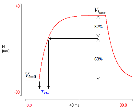
If \(t=\tau_{m}\) then \(-t/\tau_{m}=-1\). The value of e-1 is 0.37, so (1 – e-1) is 0.63. Thus when \(t = \tau_{m}\) the following is true for a spherical cell:
\begin{equation*} V_{(t = \tau_{m})} = 0.63V_{t_{max}} \end{equation*}So all we have to do is find the time from the start of the stimulus at which the voltage is equal to 63% of its final value, and we have the time constant.
- Set the simulation back to its starting conditions.
- Click Start.
Task: Calculate the membrane time constant of the cell in the simulation by finding the time at which the voltage reaches 63% of its final value. NOTE, the final voltage that we want (\(V_{t_{max}}\)) is the voltage relative to the starting voltage, not the absolute voltage. So in our simulation the absolute final absolute voltage is about +25 mV, but this is from a resting potential of -60 mV, so the voltage we want to take 63% of is about 85 mV. Then we have to add back the resting potential to get the absolute voltage we are looking for. Also, don’t forget that the stimulus starts at 10 ms, so subtract that from your time value.
Hint: You can use cursors to help find the time at which a particular voltage occurs:
-
- Add a horizontal cursor and drag it to the starting and final voltages in turn, noting the voltage values (you could also use the standard Measure facility).
- Calculate the voltage at 63% of the difference.
- Position the horizontal cursor at that voltage.
- Add a vertical cursor and position it where the horizontal cursor crosses the voltage trace.
- Read the time of the vertical cursor, and subtract the time of the start of the stimulus.
- You now have the value of \(\tau_{m}\).
Additional Task: Can you reconcile your measured time constant with the parameters in the Passive Properties dialog (i.e. is your measured value equal to RC)? It doesn’t matter whether you use the area-specific values (per cm2) for resistance and capacitance or the absolute values, the area units cancel out (see below). But it does matter that you get the units right, and that you use resistance not conductance values to calculate RC.
The Falling Phase
The equation describing the falling phase of the response is rather simpler:
\begin{equation} V_{t} = V_{t=0}e^{-t/(\tau _{m})} \label{eq:eqFallingExp} \end{equation} Now t is the time after switching off the stimulus, so Vt=0 is the peak voltage achieved during the stimulus. Equation \eqref{eq:eqFallingExp} is actually the standard equation for any decaying exponentialIn school maths textbooks this is often give as A=A0ekt. For us, A is V, and k is -1/τ., and the rate of decay is governed by the single factor, the membrane time constant, \(\tau_{m}\).
Task: Measure the time constant \(\tau_{m}\) from the falling phase of the voltage trace (i.e. after the stimulus switches off).
We could measure \(\tau_{m}\) by finding how long it takes to decay to within 37% of its final value (like the 63% for the rising phase), but there is another way - we can get the time constant from the slope of a graphical plot of the logarithm of voltage against time. This is apparent from the log transform of equation \eqref{eq:eqFallingExp}:
\begin{equation} \ln(V_{t})=-\frac{1}{\tau _{m}}t +\ln(V_{t=0}) \label{eq:eqLnExpDecay} \end{equation}
which is linear against t with slope \(1/\tau _{m}\)
-
- Set the left-hand X axis scale to 50 ms. This sets the start of the Results display to the time when the stimulus is switched off.
- Click the drop-down arrow on the Copy button and select Copy text. This copies the raw data values that are displayed on the screen to the clipboard.
- Open Excel or a similar graphing program, and paste in the data.
- Make a plot of the time from switching off the stimulus (X axis) against the natural logarithm (base e) of the relative voltage values (Y axis)
Important: Before plotting, you will need to do some data transforms. You need to make the initial time (switch-off time) 0, so subtract 50 from all time values. Also, you need to make the voltage values relative to the resting potential (-60 mV), so add 60 to all voltage values before converting them to their logarithm. - The graph should be a straight line, and the negative of its slope should be the reciprocal of the time constant.
Time Constant is Size Independent
Earlier on you changed the cell diameter and found a dramatic change in input resistance. However, if you were to measure the time constant, you would find that its value stayed the same. This is because resistance is inversely proportional to surface area, but capacitance is directly proportional to surface area. If you have a bigger surface area you have more conductors and hence lower resistance, but also more capacitors and hence higher capacitance. The two changes cancel each other out, and their product, the time constant, stays the same.
Temporal summation: Why the Time Constant Matters
Temporal summation is the addition of separate signals that occur in rapid succession in time. It is a crucial aspect of synaptic integration.
- Load file Passive Cell Body Temporal Summation.
- Click the Passive check box in the Setup view to call up the Passive Properties dialog box.
- Click Start.
The lower trace shows two brief stimuli following each other in rapid succession, the upper trace shows the voltage responses. The voltage starts to rise in response to the first stimulus, but it gets nowhere near its maximum steady-state value before the stimulus finishes and the voltage starts to drop again. However, the second stimulus occurs before the response to the first has returned to baseline, and the second response “adds onto the back” of the first, so that the second peak is substantially bigger than the first. This is temporal summation.
- Reduce the membrane capacitance to 1 µF (this will reduce the time constant by a factor of 3).
- Click Start.
The voltage responses are bigger (Question: Why?), but the degree of temporal summation is reduced. The second peak is not much bigger than the first.
Take-home message: The time constant has a strong influence on the degree of temporal summation that occurs with high-frequency signals - longer time constants give more summation.
Low-Pass Filter
An intuitive consequence of the RC properties is that if a stimulus current changes, then the voltage response to that change lags behind it. This is obvious with a square-pulse stimulus, where, as we have seen, the voltage reaches its peak some time after the stimulus itself peaks. This means that if the stimulus changes repeatedly, the voltage never manages to reach the peak which it could attain if only the stimulus remained stable long enough for it to catch up! So high frequency (rapidly changing) signals are attenuated as well as delayed.
- Load and Start the file Low-Pass Filter.
- This simulation uses the Network module so the interface looks a bit different, but hopefully the following instructions are clear.
The initial experiment applies a simple, long-duration square pulse stimulus (lower trace) to a neuron with purely passive membrane (no voltage-dependent channels). As we have seen several times before, the membrane potential (upper trace) rises to a peak stable value determined by the input resistance.
- Click the Sine wave radio button in the Experimental control at the left of the Setup view. (The simulation runs immediately because Options: Run on change was preselected.)
The stimulus now changes to a sine wave with a period of 100 ms (10 Hz frequency), and it generates a voltage response which is also a sine wave of the same frequency. However, while the stimulus has exactly the same peak amplitude as before, the peak of the voltage response does not quite reach the same level as it did for the square pulse.
- Change the Period of the sine wave to 20 ms (50 Hz frequency) by editing its value in the Experimental control.
The stimulus still has the same peak amplitude, but the peak of the voltage response is now considerably below what it was for the sine wave with the 100 ms period.
It is not just the amplitude of the voltage that is changed, but also the timing.
- Click the Measure check box in the Results view, and drag the dialog away from the trace display.
- Drag the red cursor so that it lines up with the first (and only) peak in the 10 Hz stimulus (not voltage) trace. This should also line up with the second peak of the 50 Hz stimulus trace.
Note that the peaks of the voltage responses to both the 10 and 50 Hz input lag behind the peak of the stimulus.
Phase Delay
A lag expressed as a fraction of the cycle period is known as a phase delay.
Task: Calculate the phase delay in the voltage response to the stimulus with the 20 ms cycle period (50 Hz), and then to that with the 100 ms cycle period (10 Hz).
-
- Without clearing the screen, set the start time (X axis left scale) to 30 ms and the end time to 50 ms to "zoom in" the display to see the timing in detail.
- For the top axis, set the top scale to -25 mV and the bottom scale to -75 mV to see the peaks of the voltage waveform more clearly.
- Set the Highlight sweep value to 3, to focus on the 50 Hz traces.
- Click the 2 cursors check box in the Measure dialog, and then click the Only difference check box.
- Drag the blue cursor to align with the peak of the sinusoidal stimulus (shown in the lower axis at about 35 ms).
- Drag the red cursor to the peak of the 50 Hz voltage trace (at about 38.2 ms).
- Click Measure in the dialog.
- The value in the time column of the measurements is the red-blue difference, which is the lag between peak stimulus and peak response.
- Set the Highlight sweep value to 2, to focus on the 10 Hz traces.
- Drag the red cursor to the peak of the 10 Hz voltage trace (at about 39.8 ms).
- Repeat the measurement.
- Calculate the phase delay (lag/period) for the two frequencies.
- Without clearing the screen, set the start time (X axis left scale) to 30 ms and the end time to 50 ms to "zoom in" the display to see the timing in detail.
You should find that there is a much greater phase delay with the higher frequency stimulus.
Together, these properties mean that the membrane acts like a low-pass filter – i.e. a signal processing component that allows low-frequency signals to pass through it more readily than high-frequency signals.
Take-home message: The RC properties mean that the voltage response to a rapidly changing stimulus is smaller than that to a slowly changing stimulus, and the peak of the response lags behind the stimulus in a frequency-dependent manner, with higher frequencies having greater phase delay.
Axons and Dendrites: Conduction of Passive Signals
When current is injected into a spherical cell, it can only go into the membrane capacitor, or back out of the cell through membrane ion channels like the leakage channels, it has nowhere else to go.
However, if current is injected into a dendrite or axon, there is a third option: the current can spread inside the cell along to the next section of the structureOf course, a real dendrite or axon is continuous and doesn’t have arbitrary “sections”. But it makes it easier to conceptualize if we think of each short length as a separate section. And, as we will see later, dividing a structure into small isopotential sections is the basis of compartmental modelling.. When it arrives in this second section, there are again 3 choices: into the capacitor, out of the cell through ion channels, or along the cell into the third section. However, the current available is now less than the original because some current has already been "used up" in the first section through charging the capacitance and loss through ion channels, so the voltage change produced by current in the second section is less than that in the first. Similarly, the voltage change in the third section will be less than the second, and so on. At each section some current is lost, and so the remaining current entering the next section is less and less, until eventually there is no interior current left, and there is no voltage change.
It is a bit like water leaking out of a hosepipe with a series of holes in it:

This means that an extended cell form like a dendrite or axon is no longer isopotential in response to a stimulus. A stimulus signal injected at one point spreads along the structure, but as it spreads it varies with both time and distance. Specifically, it is both delayed and attenuated.
Note: the Passive Conduction model used in the following simulations does not include the resting potential: all voltages start off at 0. You can just imagine that -60 mV is added to everything, if you want.
Attenuation and Delay: Basic Properties
We’ll start by injecting a square current stimulus into a passive dendrite.
- Load file Passive Conduction.
The top part of the Setup view shows a section of dendrite with a fixed stimulating electrode for injecting current (oblique green triangle at the left end) and a moveable recording electrode (vertical red triangle) for recording the voltage response at different locations on the dendrite. The two electrodes start off in the same position on the dendrite.
The bottom part of the view shows the dendrite properties. The dendrite is assumed to extend a long distance on either side of the electrodes, and has uniform properties over its entire length (which of course is biologically unrealistic, but it allows us to establish basic principles without having confusing anatomical details).
- Click Start.
At first sight the overall response in the Results view looks very similar to that of the spherical cell. Without clearing the screen:
- Set the recording electrode position E1 to 1 mm. This can be done by clicking the up spin button.
- A new simulation starts automatically because Options: Run on change has been pre-selected.
Note that the red triangle moves along the dendrite so it is now 1 mm away from the stimulation site. The voltage response is weaker and slower rising.
- Repeat at distances of 2, 3, 4 and 5 mm.
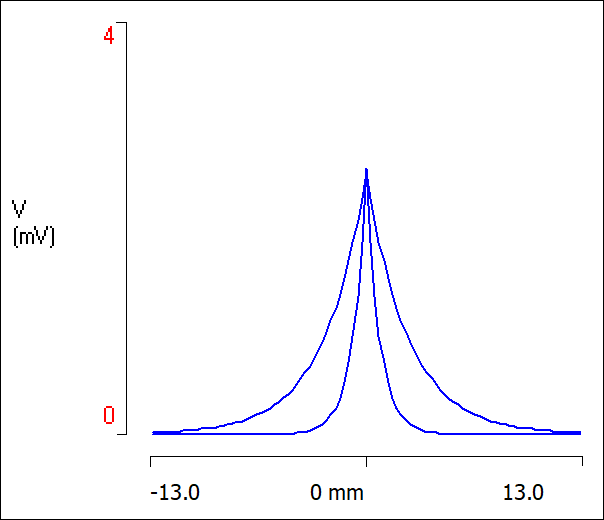
Your screen should now look like this:
It is obvious that the further the recording is from the stimulation site, the lower the final voltage (this is attenuation with distance), and the slower the rate of rise (this is increased delay with distance).
The Space (Length) Constant: Attenuation with Distance
First we will investigate how the voltage attenuates with distance.
- Click the Measure button in the Results view to show the Measure dialog.
- Drag the red measure cursor until it is over the highest voltage, just before the end of the stimulus. It may not need moving much.
- Click the Measure button within the dialog (not on the Results view).
The dialog measures the voltages at the time of the cursor location for all 6 simulation runs simultaneously.
- Click +User in the Measure dialog to insert a column at the left.
- Edit the user column header to read Distance (mm) (this is not essential, but it keeps things clear).
- In each row of the user column, enter the distance of the recording electrode from the stimulus electrode for that measurement (i.e. the numbers 0 to 5).
- Click the Plot button in the dialog.
- Select E1 from the Y axis drop-down list.
The plot shows how the voltage decays with distance from the site of current injection. The decay looks like it might be exponential, but it is hard to tell for sure.
-
- Check the Log Y box in the plot (XY Scatter) dialog.
- Click the radio button choice e to select the natural logarithm (as opposed to log base 10). This doesn't change the shape of the plot, but it does change the numbers.
The plot now shows a straight line, which confirms that the decay is indeed exponential (see equation \eqref{eq:eqLnExpDecay}).
The equation for exponential decay with distance can be writtenThis equation is similar in form to that for the falling phase of the time constant \eqref{eq:eqFallingExp}, but operates in space rather than time.:
\begin{equation} V_{x}=V_{0}e^{-x/\lambda} \label{eq:eqSpaceConst} \end{equation}where x is the distance from the site of current injection. The rate of fall is governed by just one factor, \(\lambda\) (lambda), which is called the space or length constant and has units of distance. As before \eqref{eq:eqLnExpDecay}, the decay factor \(\lambda\) can be determined from the slope of the line of the log plot.
Task: Calculate \(\lambda\). .
- Check the Linear trendline box near the bottom of the plot dialog.
- Note the value of the Slope that appears under the checkbox.
The negative reciprocal of the slope is the value of \(\lambda\). It should be close to the space constant parameter value of 2.5 mm which is visible in the Derived Parameters group in the lower part of the Setup view.
- Close the Plot and Measure dialogs.
Voltage vs Distance Display
- Click Clear in the Results view.
- Increase the duration of stimulus Pulse 1 to 100 ms, so that the stimulus lasts for the whole display time.
- The simulation should run immediately you change the duration.
Note the “heat map” of the dendrite in the upper part of the Setup view. This illustrates the way the signal declines in amplitude as it propagates away from the site of current injection.
- Click Clear.
- Change the axon scale (at the right-hand end of the axon in the upper Setup view) from 5 to 13 mm.
- In the Results view, select the Volt vs Distance option in the Display mode group.
- Click Start.
The Results view now shows a plot of the voltage at every point along the dendriteYou couldn’t practically do this with microelectrode recordings, but you might just manage it with some sort of voltage-sensitive dye., with the centre of the display being the site of stimulus injection. So we are seeing both sides of the dendrite here, whereas in the Setup view we only see the dendrite to the right of the stimulus site.
We can see the exponential decline with distance on either side of the central point. The voltage has declined to about zero by the edges of the display, which represents a distance of about 5 space-constantsAs a useful rule of thumb, bounded exponentials reach their final values in about 5-6 decay constants. (5 x 2.5).
Diameter Affects the Space Constant
If membrane properties stay constant, changing the diameter of a dendrite or axon changes the space constant: small-diameter axons have shorter space constants.
- Load the file Space Constant and click Start.
This should just get us back to where we were at the end of the last activity.
- Set the axon diameter to 2.5 µm. I.e., reduce the diameter by a factor of 10.
- Reduce the amplitude of stimulus 1 to 0.032 nA.
We need to reduce the stimulus because smaller diameter dendrites have a higher input resistance and so will have a bigger voltage response to the same stimulus, but we want to keep the peak voltage the same as with the larger axon so we can make a comparison. I found the value by trial-and-error; it is not one-hundredth of the original as it would be for a spherical cell (see Input Resistance below). - Click Start.
The voltage profile now declines much more sharply, as seen below.
- In the Results view, set the Highlight sweep value to 1, then 2, to see the two responses separately.
The narrower response profile is reflected in the value of the space constant in the Derived Parameters of the Setup view, which is now only 0.79 mm.
Why is the Space Constant Diameter-Sensitive?
Intuitively, we can see that the space constant is influenced by the ratio of membrane resistance to internal resistance. If the membrane resistance is relatively high, then the current will spread further inside the dendrite before it all leaks out. Alternatively, if the internal resistance is high, the current will tend to be pushed out across the membrane in preference to spreading internally.
It can be shown (although it is beyond this tutorial) that the space constant can be expressed mathematically in terms of membrane and intracellular resistance or conductance:
\begin{equation} \mathsf{Length\;(space)\; constant}\; \lambda = \sqrt{\frac{r_{m}}{r_{i}}} = \sqrt{\frac{g_{i}}{g_{m}}} \label{eq:eqLamdaResRatio} \end{equation}where rm is the total membrane resistance of a 1 cm length of the dendrite, and ri is the total internal resistance of that same length, and gm, gi are the conductance equivalents. (See Passive Units for the relationship between specific and unit-length parameters.)
If you increase the diameter of the dendrite, both the membrane and internal conductance values increase, but the internal conductance goes up more than the membrane conductance, hence the length constant goes up. This is because the internal conductance is proportional to the cross-section area of the dendrite and hence the square of its diameter, while the membrane conductance is linearly proportional to the circumference and hence the diameter of the dendrite.
This is illustrated in the diagram below, where the orange boxes are ion channels in the membrane contributing to the membrane conductance (viewed side-on), and the blue circles are (imaginary) conductances in the axoplasm contributing to the internal conductance (viewed end-on).
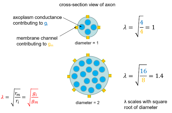
The diagram shows that doubling the dendrite diameter produces a 1.4-fold (√2) increase in the space constant. There is thus a law of diminishing returns in terms of using an increase in diameter to increase space constant.
- Set the dendrite diameter to 25 µm.
- Note the 2.5 mm value of the space constant shown in the Derived Parameters group.
- Set the diameter to 400 µm, which is a 16-fold increase.
- Note that the space constant has increased to 10 mm, which is only a 4-fold increase.
Spatial Summation: Why the Space Constant Matters
The space constant is an important parameter for passive conduction because it quantifies the rate at which a signal attenuates with distance. It has units of distance, and a typical value would be something like 5 mm.
The space constant has a major impact on spatial summation of synaptic inputs. Dendrites with a long space constant will allow synaptic inputs occurring at relatively distant sites on a dendrite to send a signal which can still reach the spike initiating zone and trigger an action potential.
Conduction Velocity
The space constant also has an important influence on the conduction velocity of nerve impulses in axons. Large diameter axons will propagate local circuits further than small diameter axons, and allow action potentials to be initiated more rapidly along the axon. In myelinated axons it also allows greater spatial separation of the Nodes of Ranvier, which again speeds conduction.
The Time Constant: Time Delay with Distance
- Load file Passive Delay and click Start.
We now see 5 simultaneous recordings made from electrodes placed progressively more distant from the stimulation site. The traces are all displayed on the same axis so that they can be easily compared. (Note that the trace and electrode colours match, but that they are just for identification, they are NOT coded to indicate voltage.)
- Note the values of the Derived Parameters (time constant = 10 ms, space constant = 2.5 mm and input resistance = 2.55 MΩ).
- In the lower Setup view set the membrane capacitance (Cm) to 2 µF (i.e. double it).
- Note in the Derived Parameters that the time constant increases, but the space constant and input resistance are unchanged.
- Click Start.
Just as with a spherical cell, doubling the membrane capacitance doubles the membrane time constant, which is now 20 ms.This slows the rate of rise of the voltage but does not affect its final value (as indicated by the unchanged input resistance). Nor does it affect the degree of attenuation, so the space constant is independent of capacitance (which is obvious anyway from equation \eqref{eq:eqLamdaResRatio}).
- Click Clear followed by Start to get just one sweep displayed.
- Set the right-hand time base axis to 40 ms, to zoom in on the first part of the stimulus.
The topmost red trace is from the electrode located at the stimulus site, and here the voltage rise looks a bit like the exponential rise of the spherical cell simulation. However, it is actually more rapid than a pure exponential. (You could do a log plot of the falling phase as you did for the spherical cell to confirm that it does not generate a completely straight line.)
As you look at progressively more distant recording electrodes, you can see that not only is the rate of rise slower, but it changes shape - the waveform becomes sigmoid. At the most distant recording, 5 mm from the stimulus site, the initial waveform is actually pretty-much flat and the rise is very gentle indeed. The waveform is clearly not exponential.
This means that our method of measuring time constant as the time taken for the voltage to reach 63% of its final value is no longer valid. The membrane still has a time constant, and that constant is defined as before:
\begin{equation} \mathsf{Time\; constant}\; \tau_{m} = R_{m}C_{m} \label{eq:eqTimeConstDef} \end{equation}but it cannot easily be measured because the waveform is distance-dependent.
- Re-loadThe easiest way to re-load a parameter file is to select it from the first entry in the File: MRU (most recently used) list below the Notes command. Passive Delay to return to the starting conditions.
- Click Start.
- In the lower Setup view set the membrane resistance (Rm) to 20 (i.e. double it).
- Click Start.
Now the time constant, input resistance and space constant are all increased. The same amount of current generates a larger final response at all positions along the axon. This makes sense because reducing the “leakage” across the membrane means that the current will spread further inside the axon before it leaks away.
Temporal Summation: Why the Time Constant Matters
We have already seen the effects of the time constant on temporal summation in a simple spherical cell. What happens if we add in the complication of passive conduction?
- Load file Passive Conduction Temporal Summation and click Start.
The bottom trace shows two brief stimuli following each other in relatively rapid succession. The top (red) trace shows the voltage response at the site of current injection. There is very little temporal summation – the second peak is not much bigger than the first.
The middle (purple) trace shows the voltage response two space-constants away. The response is much smaller, as we would expect due to attenuation (note the different axis scales), but now the two responses do interact, and the peak of the second response is considerably greater than the peak of the first. So temporal summation is occurring away from the site of current injection, but not actually at the site.
- Increase the membrane resistance (Rm) to 20 (i.e. double it).
- Click Start.
The response at the site of current injection (E1) is very similar, but the temporal summation at the distal site on the dendrite (E5) is considerably enhanced.
Question: Given that the current stimulus is the same in both situations, why does the increase in membrane resistance cause so so little change in the voltage response at the site of current injection, and yet such a substantial change a few millimetres further along the dendrite?[Hint: I don't think there's an easy answer to this - it just comes out in the mathsWhich is one of the joys of simulation - you can find out things that are not intuitively obvious.. So notice it, and think about it's consequences, but don't spend a long time worrying about its cause.]
Take-home message: Passive conduction can cause different degrees of temporal summation at different regions in a dendrite.
Input Resistance
We have already noted that the input resistance in a dendrite or axon does not have the simple square-root relation to axon diameter that we found in a spherical cell. This is because current entering the structure can spread sideways within the cell, as well as just leaving through the immediate membrane resistance.
I will not derive it, but the input resistance follows this equation:
\begin{equation} \mathsf{Input\; resistance\;} = 0.5 \sqrt{r_{m}r_{i}} \label{eq:eqCableInputRes} \end{equation}See Passive Units for definitions of unit membrane resistance \(r_{m}\) and unit axoplasmic resistance \(r_{i} \). The unit resistance is the resistance (either membrane or axoplasmic) of 1 cm length of the axon or dendrite in question.
The Cable Equation
You REALLY don’t have to be concerned with the equation that underlies the passive conduction waveforms given above in order to understand the physiological significance of the process, but in case you are interested, here it is:
\begin{equation} \begin{aligned} V(T,X) = \frac{{{r_i}I\lambda }}{4} \Bigl\{ & e^{ - X}\left[ {1 - \textrm{erf}\left( {\frac{X}{{2\sqrt T }} - \sqrt T } \right)} \right] - \\[1.5ex] & {e^{ - X}}\left[ {1 - \textrm{erf}\left( {\frac{X}{{2\sqrt T }} + \sqrt T } \right)} \right] \quad \Bigr\} \end{aligned} \label{eq:eqCableEqn} \end{equation}This rather intimidating equation is given by Jack, et al., (1975; equation 3:24), and was originally derived (in modified form) by Hodgkin & Rushton (1946). It gives the voltage V at any time T after the onset of injection of a current of constant amplitude I, at any distance X from the site of injection. X and T are distance and time parameters which have been "normalised" against the membrane parameters of space and time constant; i.e. \(X=x/\lambda\), \(T=t/\tau_{m}\), where x and t are real distance (in mm) and time (in ms) respectively. The function 'erf', which is called the error function, is a function with a defined distribution just like other, better known, functions such as the exponential or sine functions.
The equation above gives the voltage change following the onset of a current pulse. The voltage decay following the offset of current is achieved by symmetrical superposition, i.e. adding a second, negative current pulse at the appropriate time.
The limitation of the equation is that it assumes that the axon/dendrite is infinitly long, and has uniform properties throughout. This means that it is a useful starting for conceptual exploration, but a more complicated approach is needed to model real structures.
Non-Uniform Diameter: A Compartmental Model
Many axons are reasonably uniform in diameter, but dendrites are usually not. This means that they have space and time constants that vary along their length, and the cable equation \eqref{eq:eqCableEqn} given above cannot be used. In fact, there is no explicit formula that allows you to calculate the voltage response of a non-uniform dendrite at an arbitrary position, you have to build a compartmental model if you want to investigate this.
- Load file Non-Uniform Dendrites.
- Note that this uses the Network model, so the interface is different from that seen previously in this section.
Four segments of dendrites are shown aligned vertically in the Setup view. Each dendrite is made up of several compartments that show as circular blobs. The size of the blob is an indication of the dendrite diameter, but it is not drawn to scale.
The dendrite on the left (A) has a uniform diameter of 50 µm. The second dendrite (B) starts off at 25 µm diameter but then expands to 50 µm, the third dendrite (C) starts of at 50 µm but then contracts to 25 µm, while the dendrite on the right (D) has a uniform diameter of 25 µm. The total length of each dendrite is 400 µm, and for simplicity the diameter change occurs as a step in a single location 150 µm from the top on the dendrite.
A stimulus is applied to the top compartment in each dendrite.
- Click Start.
The upper set of Results traces show the voltage responses at the site of the stimulus. The strength of each stimulus has been adjusted so that the final voltage at this position is virtually the same in each dendrite, but note that the time course with which this voltage is approached differs slightly between the dendrites.
The lower set of traces shows that the voltage response at the end of the dendrite is very different between three of the dendrites. The uniform thick dendrite (A) has the biggest final voltage (red trace). This is perhaps not surprising because it has the largest average diameter of the four, being entirely made up of large-diameter compartments, so one would expect it to have the longest space constant.
However, the next largest response (green trace) is from dendrite (C), that starts wide but then narrows. The smallest responses are from the uniform narrow dendrite (D) , and the dendrite that starts narrow but then widens (B). The (B) result is at first sight surprising, since the average diameter of that dendrite is greater than either the narrowing or uniform thin dendrite.
Take-home message: Attenuation in a tapering dendrite depends on the direction of taper. Input at the narrow end of an expanding dendrite produces a much weaker signal at the terminal than input at the wide end of a narrowing dendrite.
Spatial Summation
A key feature of passive conduction is that it allows signals to summate: i.e. to add together, either positively or negatively. This means that an array of passive dendrites can integrate information from multiple sources occurring at the same or slightly different times. The end numerical "result" of this integration is the membrane potential at the spike initiating zoneThe axon hillock is the spike initiating zone in a vertebrate motorneuron, but it may have different locations in other types of neurons.: if this exceeds threshold then a spike is initiated, if it does not, no spike occurs. Thus the properties of passive conduction lie at the heart of decision making in the nervous system, and passive conduction should very definitiely not be regarded as the poor relation of spike conduction.
- Load the file Spatial Summation.
The Setup view shows a schematic motorneuron implemented as a compartmental model. There is a cell body (soma) shown as a purple blob, with an axon sprouting off it at the top, bending to the right (the axon is obviously truncated, but this is just a concept model and is not meant to be anatomically realistic). The axon can maintain Hodgkin-Huxley-type spikes, but the soma is passive. Three passive dendrites sprout from the soma and spread downwards in the view. Each dendrite receives excitatory synaptic input at its distal terminal, from separate pre-synaptic neurons. The soma itself receives inhibitory synaptic input from a fourth pre-synaptic neuron. The pre-synaptic neurons can be activated by experimental stimuli (the square boxes labelled 1 - 4).
The neurons are colour-coded by their membrane potential - their dark blue colour indicates that they are currently at rest.
- Click Start.
None of the pre-synaptic neurons is being stimulated, so all neurons remains at rest.
Additive Spatial Summation
- With stimulus 1 selected (which it should be by default when the file is loaded), click the up arrow of the Amplitude spin button to set the stimulus to the left dendrite excitatory pre-synaptic neuron to 10 nA.
Run on change is pre-selected, so a simulation sweep occurs immediately. The left excitatory pre-synaptic neuron spikes in response to the stimulus (shown in the pre-syn bottom trace) , and generates an EPSP in the distal compartment of the left dendrite (post L trace). This spreads by passive conduction to the soma where a positive deflection is visible (soma trace), but the potential is below threshold at the adjacent axon hillock, so no spike is generated.
- Select stimulus 2, either in the list on the Experimental control panel, or by clicking the stimulus box in the Setup view.
- Click the amplitude up spin button.
The mid excitatory pre-synaptic neuron spikes in response to the stimulus (shown in the pre-syn bottom trace, but note that for clarity the simulus is slightly delayed relative to the first so that the spikes do not completely overlap. This generates an EPSP in the distal compartment of the mid dendrite (post M trace). This spreads by passive conduction to the soma where it combines with the EPSP generated on the left dendrite to produce a bigger positive deflection.
This is spatial summation! Two inputs have occurred virtually simultaneously, but on two different spatial locations on the neuron. Both inputs spread by passive conduction to a summation point (the soma), where they add together.
However, the summed response is still below threshold.
- Select stimulus 3.
- Click the amplitude up spin button.
Now the summed input at the soma is enough to take the adjacent spike initiating site (the axon hillock) above threshold. A spike is generated, and this propagates along the axon. The spike in the terminal axon compartment is shown in the top trace (end axon). It is also worth noting the "backwash" potential generated by the spike that propagates by passive conduction back out the dendrites, to produce a bump on the falling shoulder of the EPSPs.
- Click Clear, and then click Start again, but this time watch the pretty colours in the Setup view. You may want to set a Slow down factor to help you observe the timing of the potential conduction within the post-synaptic neuron.
Backwash
Note that when the neuron spikes, a "hump" appears on the falling phase of the EPSPs in the three dendrites. This is due to the spike potential propagating through passive condution out along the dendrites, and is known as spike backwash.
Subtractive Spatial Summation
- With the Results view showing an episode of spike generation, select stimulus 4 and click the amplitude up spin button.
Now the inhibitory pre-synaptic neuron generates a spike, and the consequent IPSP sums negatively with the summed EPSPs at the soma and counteracts them. This shows that spatial summation can be additive or subtractive.
You may wonder why the inhibition has been targeted to the soma, rather than a distal dendrite. The simulation could, in fact, have done the latter (and you could try it by dragging the inhibitory b synapse symbol from the soma to a dendrite terminal), but proximal inhibition is much more effective than distal inhibition. The reason for this is explored in a later tutorial.
Temporal Synchrony
The preceding tutorial section is flagged as spatial summation, but in fact you cannot have effective spatial summation unless there is also temporal synchronization. If two inputs happen at widely separate times, then they cannot summate because the effect of one is over before the other arrives at the summation point.
- Clear the Results view and click the amplitude down spin button for stimulus 4 to turn off the pre-synaptic inhibitory neuron.
You should now again see additive summation producing a spike.
- Select stimulus 3.
- Click the up spin button for the Delay, to delay activation of the right excitatory pre-synaptic neuron by 5 ms.
The EPSP from the right dendrite now arrives at the soma too late to sum effectively with the EPSPs from the other dendrites, and no spike is produced. (Use the Highlight sweep facility to sort out the two conditions if you are confused by the overlaid traces in the Results view).
Hopefully this illustrates that spatial summation and temporal synchronization interact with each other, and that the former cannot be effective without the latter.
I am avoiding using the term temporal summation here, because that usually refers to the situation where a single pre-synaptic neuron is activated several times in rapid succession. Then the later EPSPs can sum with the earlier ones to produce a larger overall potential (this was covered in an earlier tutorial). The summation occurs at the immediate post-synaptic site, and it is this summed potential that spreads to the overall summation point, where it may interact through spatial summation with inputs occurring at other locations.
Take-home message: Spatial summation occurs when multiple near-synchronous synaptic inputs arrive at different spatial locations within the dendritic field of a post-synaptic neuron. The PSPs spread by passive conduction to the spike initiating zoneActually, in a non-spiking local interneuron there is no spike initiating zone because there are no spikes. Instead, each synaptic output site acts as an integrating region, and its local membrane potential determines the synaptic output of the neuron at that site. where they are integrated to produce a single membrane potential that determines whether a spike is generated.
On to Action Potentials (Spikes) ...