Copyright © W. J. Heitler (2019)
Kinetics of Single Ion Channels
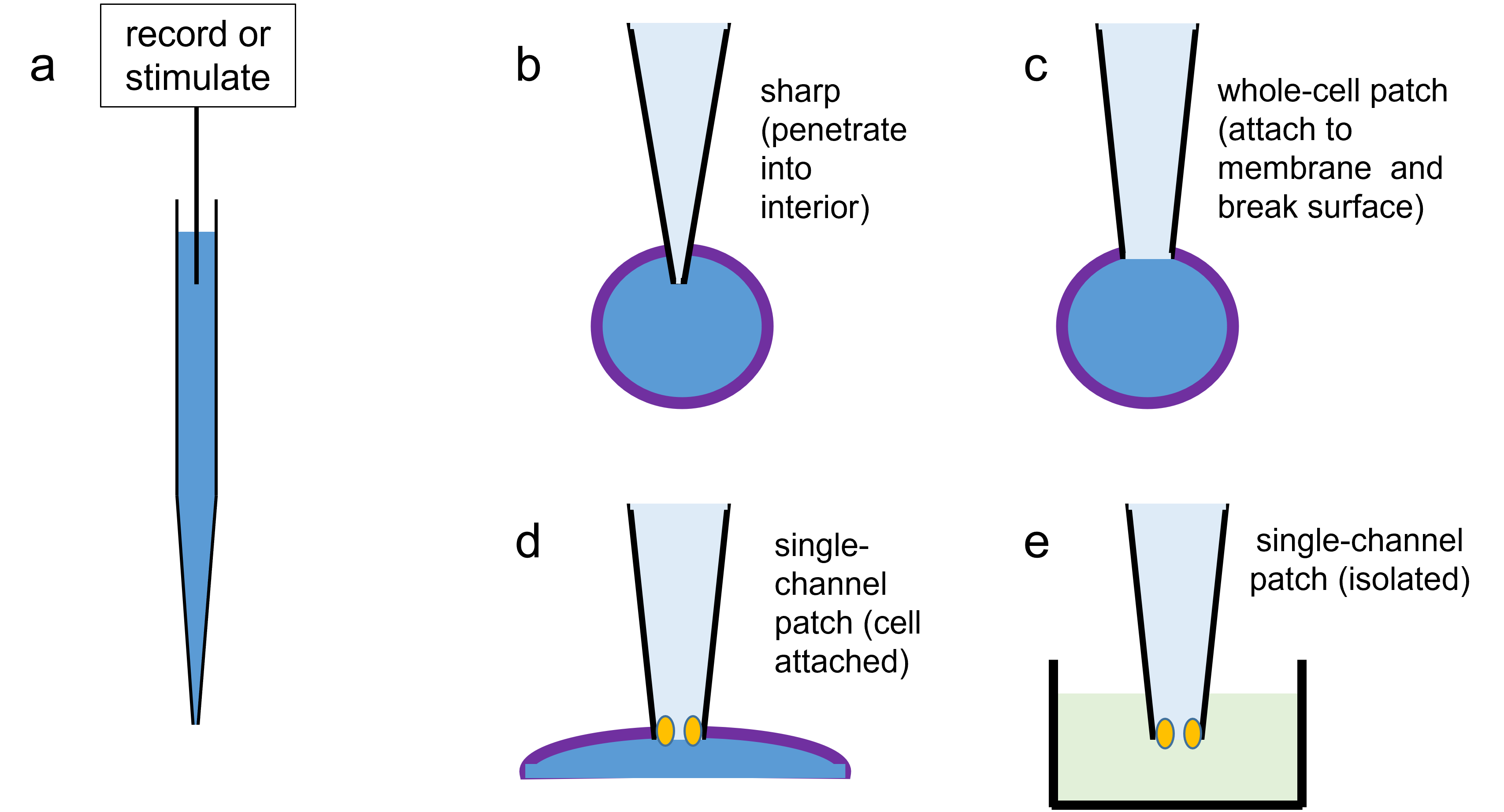
The patch clamp recording technique can measure the flow of current through a single ion channel in a patch of membrane, and hence the conductance of that channel. In most cases the conductance switches between two states – open and shut, with no intermediary levels. In kinetic analysis the information contained in the timing of these changes in conductance is used to deduce information about the molecular mechanisms that bring them about.
Kinetic analysis of single channel recordings is a fairly intimidating topic for most non-biophysicist neurobiologists (including the author). One of the best summaries of the topic that I am aware of, which gives enough information to be of practical use, without completely swamping the non-mathematician, is contained in Colquhoun & Hawkes (1994). A lot of the explanatory details given below follow the lines of reasoning developed in that article. More details, including a fuller mathematical treatment, are contained in Colquhoun & Hawkes (1983). Finally, Colquhoun & Hawkes (1981) do us the considerable favour of giving two fully-worked numerical examples. It was some relief to the author to find that the Neurosim simulations yield the same results as the explicit analytical approach taken in that paper (at least, they do now, after a few false starts...).
This chapter considers 4 main types of kinetic schemes:
- A two-state open/shut channel.
- A two-state channel in the presence of a blocking antagonist.
- A three-state channel that requires an agonist to bind to it in order to open.
- A model of the nicotinic acetyl choline channel that requires 2 molecules of ACh to bind to it in order to open.
An Open-and-Shut Case (2-State Channel)
- Switch to the Membrane Patch model by selecting from the Model menu command, or making the appropriate choice at programme start-up.
In the Setup view, the pictures in the grey box entitled Simple Model show an ion channel with a single gate in it. The gate can be in one of two states, open or shut, and the conductance state of the channel itself is simply determined by the position of the gate.
- Click the Start button to run an experiment. [You may need to increase the Slow down factor on the main toolbar.]
- After a while, click Pause so that you can read on.
At the bottom left of the Results view you should see a cartoon of the channel with a single gate in it, and the gate should open and shut. When it is open, an arrow is drawn through the channel to indicate that it can allow ions through. At the bottom right of the view is a state graph showing two states, open and shut - this refers to the gate. Above that is a conductance graph, showing two levels, high and low - this refers to the channel. When the gate is open, the channel has a high conductance, when the gate is shut, the channel has a low conductance. In this simple model, the conductance level and the molecular state have a very direct relationship (which is why it is simple), but as we shall see, this is often not the case. As the simulation progresses, note that the Open count, shown to the left of the Results view, increments by 1 for every transition made by the channel from the closed to the open state. At this point do not worry about what the rest of the Results view shows, but read on.
Mean Sojourn Duration and Transition Rate Constants
The gate in the channel opens and shuts randomly. If the gate is open, it has a certain probability of shutting. This probability is expressed as a transition rate constant (\(\alpha\)), with units of s-1 (i.e. per second). Conversely, if the gate is shut, it has a certain probability of opening, again expressed as a transition rate constant (\(\beta\)).
\begin{equation} \ce{open <-->[\alpha][\beta] shut} \label{eq:eqAlphaBeta} \end{equation}How do we interpret \(\alpha\) and \(\beta\)? The value of \(\alpha\) tells us that for every second that the channel is in the open state, it will on average shut \(\alpha\) times. Conversely, for every second that the channel is shut, it will on average open \(\beta\) times. [NOTE: \(\alpha\) and \(\beta\) have the opposite meanings to the way they are used in the Hodgkin-Huxley equations. This is unfortunate, but it’s the convention and we have to live with it.] In the present experiment, \(\alpha\) = 1000, \(\beta\) = 250 (look at the Setup View to check this). Of course, to accumulate 1 second of open time which has many shutting episodes in it (on average, 1000) will take longer than 1 second of actual real time, because of the intervening periods of shut time, but nonetheless, if the gate shuts on average 1000 times for every second that it is open, it means that the average length of time that the gate is open is 1/1000 seconds, or 1 ms.
Take-home message: In a simple open or shut channel, the average length of time a channel stays in a particular state (the sojourn in that state) is the reciprocal of the transition rate constant that leads out of that state.
In the simple model there is only one rate constant out of each state (\(\alpha\) out of the open state, \(\beta\) out of the shut state), but we will deal with more complex situations later. In the simple model with these transition rate constants, the average (mean) duration of the sojourns in the open state is thus 1/\(\alpha\) = 1 ms and the mean duration of the sojourns in the shut state is 1/\(\beta\) = 4 ms.
- Click Continue to resume the experiment.
Look at the conductance level graph. It should become obvious after a time that although individual open and shut sojourns are highly variable, on average the shut sojourns are considerably longer than the open sojourns. When you have got fed up with watching the state and conductance graphs at the bottom of the screen (or when you think you understand what they show):
- Check the box labelled Fast above the cartoon in the left of the Results view.
This makes the simulation run as fast as possible, so everything freezes except the open count, which keeps you informed about how the experiment is progressing. When the experiment has accumulated 2500 shut-to-open transitions (and also 2500 matching open-to-shut transitions) the experiment stops.
Two histograms are displayed above the conductance graphs, but do not worry about their shapes yet. Just note the numerical values of the mean sojourns shown below the histograms. These will not exactly match the mean durations as defined above, because we are dealing with random probabilistic events, but with 2500 samples they should come fairly close.
Sojourn Distribution is Exponential
The probability of a channel undergoing a transition to the other state (open or closed) is completely independent of the time since the channel last underwent a transition. This means that channel opening or closing is a Poisson process. A histogram of the intervals (I) between Poisson events has a decaying exponential shape:
\begin{equation} I_{t} = I_{t=0}e^{-t/\tau} \label{eq:eqFallingExp} \end{equation}
with the time constant \(\tau\) equal to the average interval. Such a shape is called the probability density function (PDF) of the distribution. We have already seen that the average interval is the reciprocal of the transition rate constant, so equation \eqref{eq:eqFallingExp} describing the PDF can be written as:
\begin{equation} I_{t} = I_{t=0}e^{-\lambda t} \label{eq:eqSojourn} \end{equation} where \(\lambda\) is the transition rate constant (\(\alpha\) or \(\beta\)).
What does it mean to say the distribution is exponential? When a channel opens, in the majority of cases it shuts again very quickly, but in some cases it stays open for longer, and in a few cases it stays open a long time. Thus if we plot a frequency histogram of the duration of each open sojourn of the channel, there is a high bin count for short duration sojourns, and then a progressively declining bin count for sojourns with longer and longer durations. Exactly the same is true for the channel starting off in the shut condition. The peaks of the bin counts in the histogram form a declining exponential curve, and that is what is meant by an exponential distribution in channel sojourn durations.
The histogram labelled Open Time Duration should have a fairly clear exponential shape. The histogram labelled Closed Time Duration has a weirder shape, but that is because the X-axis timescale is too short. Sojourn durations too long to fit on the histogram are piled up in the right-hand bin, hence the large peak at the right of the closed-time graph.
- Edit the maximum (right-hand) X axis value of the Closed-Time histogram to show 25 ms, and the top axis scale to 600 counts.
The histogram should now have a clear exponential shape.
- Click Start several times to see how the exact shape of the histograms various due to the random nature of the process, but the overall shape (and the numerical value of the mean sojourn) remains fairly constant for each graph.
What happens if we change a transition rate constant?
- In the Setup view, change the value of \(\beta\) to 50.
- Click Start.
With Fast still selected, experiment should complete rapidly. Note that the mean sojourn for the closed time histogram as now increased to about 20 ms. You will need to adjust the histogram X axis scale to about 200 to visualize the exponential decline.
We skipped viewing the conductance state graphs because Fast was selected. However, we can still retrieve the data.
- Select the Analyse: View Open/Shut Data menu command to open the View Data dialog box.
The dialog box shows all the experimental data of conductance levels as if they had been recorded on a chart recorder, cut up into page-sized strips, and pasted into a laboratory data book. With the reduced value of the shut-to-open transition rate constant, it is clear that the channel now spends a substantial proportion of its time in the shut state.
Histogram Analysis
- Double-click the Closed-Time Duration histogram.
- Or select the Analysis: Closed-time analysis menu command.
The Sojourn Analysis dialog box opens. The obvious feature is the histogram, but it looks strange at this point. The rest of the options are quite intimidating at first, but we will approach them slowly.
At the top left you have a choice of Source, displaying either Open time or Closed time data.
- Switch between Open and Closed time and note that the histogram keeps the same general shape (which will be explained later), but that the axis values change.
- Select Closed time before moving on.
Below that the Histogram display group has 3 choices; Normal, Ln Y and LogX, sqrt (Y), with the latter selected.
- Click Normal.
The histogram now shows a standard exponential curve, with a red line drawn across the data. This line is a calculated exponential using the PDF described in equation \eqref{eq:eqSojourn} above, and by default it is drawn with a \(\lambda\) value equal to the mean sojourn of the state under consideration. The mean sojourn defining the PDF is measured from the data of the experiment that you have just run, not calculated from any underlying transition rate constants.
In the Fit Exponential PDFs just to the left of the histogram, there is a Mean value, which should be about 20 for the Closed time histogram (if b was set to 50 previously).
- Change the value in the top Exp mean to 100.
A new PDF is drawn which clearly does not fit the data.
- Click the Fit button, and note that the PDF returns to a reasonable fit.
The Fit button activates a curve-fitting routine that finds the PDF which maximizes the log likelihood of its fit to the histogram bars. (The Update 1 button produces a similar outcome in this situation, but it does not fit the PDF to the histogram, it just calculates the mean sojourn from the data and constructs the PDF from that.)
- Now click the Ln Y option in the Histogram display group.
The histogram changes so that the Y-axis is now the natural log (base e) of the counts. The exponential line should now be straight. The slope of this line is the time constant of the exponential (divide the X-axis by the Y- axis to get the units in ms for the time constant; if you divide the Y-axis by the X-axis you end up with units of ms-1, which are the units of the transition rate constant).
- Change the exponential mean value to 100 as you did before, and note how the slope of the line changes.
- Click Fit to restore the PDF
Log plots like this can be a great help in finding the parameters of exponential curves, as we shall see later. Note that in this Ln Y mode you can edit the X-axis scale, but the Y-axis scale is set automatically.
- Click the Log X, sqrt (Y) option in the Histogram display group.
The histogram now has a rather strange shape. The X axis is on a log scale, where each bin is of equal width in log units, and therefore of unequal width in real time units (i.e. not only do the bins towards the left of the histogram represent increasingly short sojourns, but they each contain an increasing smaller range of sojourn durations). The Y axis is displayed as a square-root scale of bin counts. The purpose of this rather exotic display is that the mean of the exponential appears as a peak within the histogram, which makes it easier to visualize its location. This type of display is fairly standard for kinetic analysis, and its utility will be more obvious when we have more complex types of exponential distribution.
- Change the exponential mean to 100 as you did before, and note how the shape of the curve stays the same, but its peak shifts horizontally.
- Click Fit to restore the PDF.
Note that in this Log X mode both the X- and Y-axes scales are set automatically and neither can be edited.
- Click OK to dismiss the Sojourn Analysis window.
The Effect of a Channel Blocker
- Select the Antagonist option in the Model Type frame of the Setup View. (Note that this is the third option in the list, not the second.)
This builds on the simple model by assuming a similar type of single-gated channel (although \(\beta\) is changed), but this time there is a blocking agent present. The pictures in the grey box show that the channel can be in one of three states: top picture gate shut (therefore channel shut) and blocker unbound, middle picture gate open and blocker unbound (and therefore channel open), and bottom picture gate open and blocker bound (and therefore channel shut).
- Click Start to run the experiment and observe the animated cartoon, the state graph, and the conductance graph.
The important difference is that now there are three states in the state graph; shut, open, and blocked:
\begin{equation} \ce{shut <-->[\alpha][\beta] open <-->[k+.\lbrack Antag\rbrack][k-] blocked} \label{eq:eqAntagonist} \end{equation}but there are still just two conductance levels, and these are what we can measure experimentally. Note that the blocking agent can only bind to the channel in the open state, and that when the blocker is bound, the channel cannot shut. (This is, of course, not necessarily a biological fact, it is merely the way we are arranging this model.) If you look at the transition rate constants in the Setup View you can see that there is no path going directly from the shut state to the blocked state (i.e. in effect the rate constant for this transition is 0).
By convention, the unbinding reaction is given a transition rate constant labelled k-. The binding transition rate constant is k+.[Antag]. This is the product of the fundamental chemical reaction association constant k+, measured in M-1s-1, and the antagonist ligand concentration, [Antag], measured in M. When we multiply these together we come up with the correct units for a transition rate constant of s-1.
Open-Time Distribution
- Check Fast to complete the experiment quickly.
Look at the Open-Time Duration histogram. It looks like a standard exponential shape, and we could confirm that by fitting an exponential PDF using Sojourn Analysis as before. However, the mean of the distribution shown below the histogram is no longer 1/\(\alpha\) (= 1 ms), but rather something in the region of 0.67 ms. Why is this?
If you observe the state graph, when the channel is in the open state (high conductance), it can go in either of two directions; it can either shut, or block. Thus the rate of leaving the open state is going to be dependent on some combination of two transition rate constants, \(\alpha\) and k+.[Antag]. The rule is a simple extension of the one given earlier: the mean length of time the channel stays in a particular state is the reciprocal of the sum of the transition rate constants that lead out of the state.
\begin{equation} \begin{split} \textsf{mean open time} & = \frac{1}{\alpha+ \textsf{k+.[Antag]}} \\[1.5ex] & = \frac{1}{1000 + 1 \times 500} \\[1.5ex] & = 0.67 \textsf{ ms} \label{eq:eqAntagonistOpenTime} \end{split} \end{equation}Effect of Blocker Concentration
- Increase the blocker concentration to 10 µM.
- Click Start (with Fast selected).
Note that the mean open time is much shorter (about 0.16 ms). This makes intuitive sense – with a higher blocker concentration, we would expect the channel to spend more time blocked.
In a real experiment, we would know the blocker concentration but not k+ or \(\alpha\). What could we have got from kinetic analysis?
Task: Run an experiment (use the Fast display) with several different blocker concentrations and write down both the concentration and the mean open time read from the bottom of the histogram. Convert the open time into seconds to make it consistent with the specified parameters (the value on the histogram is in milliseconds). Now plot the reciprocal of the mean open time (Y) against the blocker concentration (X). The result should be a straight line. The slope of the line is the blocker association rate constant k+, and the intercept on the Y-axis is the channel shutting transition rate constant \(\alpha\).
This is not magic; it derives directly from the formula:
\begin{equation} \frac{1}{\textsf{mean open time}} = \alpha + \textsf{k+.[Antag]} \label{eq:eqLinearAntagonistOpenTime} \end{equation}which has the same form as the standard formula for a straight line: y = mx + c.
Closed-Time Distribution is Multi-Exponential
Now we consider the distribution of closed times in the antagonist model.
- Return the Antagonist concentration to 1 if you changed it, and re-run the experiment.
- Double-click the Closed-Time Duration histogram.
- Or select the Analysis: Closed-time analysis menu command.
- Select in turn the 3 display options: Normal, Ln Y, Log X, sqrt (Y), leaving the last as the selected option.
The red line PDF is vaguely in the right area, but in no case is it a good fit to the histogram.
- Note down the numerical values of the Log relative likelihood (I had -237, but your number will vary because of the stochastic nature of the simulation) and the BIC (about 17056, again your number will vary) which are shown just above the OK button in the histogram. I will explain these shortly.
If a single exponential is not a good fit to the data, how about a dual exponential – i.e. a mixture of two single exponential distributions?
- Increase the number of exponentials to 2 by editing the value at the top of the Fit Exponential PDFs group.
Note that we now have two Proportion values, each of 0.5, and two Mean values, each of the same as the single exponential we started with. Not much improvement yet.
- Click the Fit button.
Both the Proportion and Mean values change, and the red line PDF is a much better fit to the histogram than previously.
- Select the Normal and Ln Y display options to see the fit in those modes, and then return to the default Log X, sqrt (Y) mode.
- Note that the Log relative likelihood and BIC values are now substantially smaller (closer to 0), at -21 and 16631 respectively (for my data).
Likelihood and BIC
What is the log relative likelihood? First, the likelihood. This is a measure of how likely it is that the data could have arisen from a model with the given parameters – essentially, it is a measure of the goodness-of-fit between the data and the model. The value is usually extremely small, so it is normal to express it as a logarithm, which is the log likelihood. This will be a negative number, and the closer it is to zero, the higher the likelihood and the better the fit.
A problem with likelihood is that the actual value means little outside of the context of that specific model. The log relative likelihood is the difference between the log likelihood of the current model and an unspecified "ideal" model that would produce exactly the data distribution observed. The closer this value is to 0, the better the current model is. This value can be used as a "normalized" likelihood that allows the fit of different models to be compared.
Now for BIC. If we use a more complex model, we can almost always get a better fit than with a simpler model. At the extreme, we could have a model which included parameters for every bin in the histogram, so as to exactly reproduce the observed data. However, quite a lot of the variation in the histogram is just due to random noise, and has no significance. Producing a complex model which fits the noise in the data is pointless – another experiment would produce different noise, and require a different model. This is what statisticians call overfitting. In general, one should choose the simplest model that is “good enough” in terms of its fit.
The Bayesian Information Criterion (BIC) is a numerical value that quantifies this trade-off between better fit and higher complexity. The interpretation is simple – if you have competing models with different numbers of parameters, the model that produces the lowest BIC should be chosen.
With our data the conclusion is obvious; the fit with 2 parameters is better than the fit with 1 parameter. Can we get an even better fit with 3 parameters?
- Increase the number of exponentials to 3.
- Click the Fit button.
- Observe the Log relative likelihood and BIC values.
When I tried this several times, the likelihood result varied. It was always close to that with 2 parameters, but sometimes slightly above and sometimes slightly below. But in every case the BIC value was lower with 2 parameters than with 3. So the 2 exponential model is definitely a better fit than the 1 exponential model, and the increased complexity is worthwhile. The 3 exponential model may or may not be a better fit than the 2 exponential model, but the increased complexity is not worthwhile. We should therefore chose the 2 exponential model to best explain our data.
Why are there 2 Exponentials?
From the cartoon you can see that the channel can be in a low-conductance state as a result of either of two situations; first it may be simply shut, second it may be open but blocked. These two states have nothing to do with each other - there is no direct path from one to the other. Thus from our rule above, the mean sojourn in the shut state will be 1/\(\beta\), while the mean sojourn in the open-but-blocked state will be 1/k-. Thus the low-conductance state, which is what we detect experimentally, has a duration histogram that contains a mixture of these two exponential means. The proportion of the mixture made up from each component depends upon the relative values of the transition rate constants for entering the component state. Thus when the channel is open it can go in either direction; shut or blocked. The probability of blocking is proportional to k+[Antag], and the probability of shutting is proportional to \(\alpha\).
So to put this together with the transition rate constants in our model, within the population of closed-time sojourns we would expect a fraction p to consist of shut-state sojourns, where
\begin{equation} \begin{split} p &= \frac{\alpha}{\alpha+ \textsf{k+.[antag]}}\\[1.5ex] &= 0.67 \label{eq:eqProbMixedExpon} \end{split} \end{equation}and a fraction 1-p (= 0.33) to consist of open-but-blocked sojourns. The mean duration of the shut sojourns should be 1/\(\beta\) (= 2 ms), and the mean duration of the open-but-blocked sojourns should be 1/k- (= 10 ms).
Now go back to the Sojourn Analysis window.
- Make sure the Number of exponentials is set to 2.
- If necessary, click Fit again to recover the values.
- Look at the values for Proportion and Mean in the top two rows.
Hopefully, a Proportion of about 0.66 will have a mean of about 2 ms, while the remainder (0.33) will have a mean of about 10 ms.
Comparison of Open- and Closed-Time Distributions
It is important to understand the distinction between the open- and closed-time distributions. The open-time distribution follows a single exponential with a single time constant, because there is only one state contributing to the open-time distribution. There are two ways out of this single open state, and so the single time constant of the single exponential is made up from two transition rate constants. On the other hand, the closed-time distribution follows a double exponential with two time constants, because there are two independent states contributing to the closed-time distribution. In this case each exponential time constant derives from a single transition rate constant, because each of the two states has only a single path out of it. (Note: if the paths out of the two states each happened to have the same time constant, then the two exponentials would merge, and we could not tell that there were two states there at all.).
Take-home message: The general rules are:
- The mean state sojourn is the reciprocal of the sum of the transition rate constants that lead out of the state.
- The number of exponential components in the open-time or closed-time histogram provides a minimum estimate of the number of molecular states contributing to the histogram.
What is the Point? A Reminder
In the midst of all this it is easy to loose sight of the purpose of kinetic analysis. In a real experiment we do not know how many molecular states there are, nor what the fundamental transition rate constants are - all we have are the details of open and closed time and the concentration of any ligand. The first stage of analysis is thus usually to determine how many exponential components there are in the sojourn histograms. This gives an estimate of the minimum number of underlying states. Then from the numerical parameters of the exponential mixture, further information regarding the transition rates and molecular mechanisms can be deduced. We will now go on to discuss how this can be accomplished in more complex situations.
A Transmitter-Activated Channel
- Clear the screen and unselect Fast if necessary.
- Select the Agonist model in the Setup View.
This model, which is based on the original mechanism for the nicotinic acetylcholine receptor channel suggested by del Castillo & Katz (1957), supposes that the ion channel is continuously exposed to agonist (transmitter). The channel can then be in three states: top picture the receptor channel (R) is shut by a single internal gate, and the agonist (Ag) is free (unbound), middle picture the agonist is bound to the channel receptor site (Ag.R), but the channel is still shut by its own gate, and bottom picture the agonist is bound and the channel is open (Ag.R'). The transition equation is as follows:
\begin{equation} \ce{Ag + R <-->[k+.\lbrack Ag \rbrack][\textsf{k-}] Ag.R <-->[\beta][\alpha] Ag.R'} \label{eq:eqAgonist} \end{equation}In this model the channel gate cannot open until the agonist is bound, and the agonist cannot unbind when the gate is open.
- Load the parameter file Colquhoun Hawkes 1.
This is the first of the worked examples in Colquhoun & Hawkes (1981). It uses the Agonist model described above, but with different transition rate constants.
- Click Start to run the experiment. Observe the cartoon, state graph and conductance graph, and make sure you understand the relationship between them.
- When you have seen enough, check Fast to complete the experiment.
Open-Time Distributions
Question: Can you predict the distribution shape and parameters for the open-time distribution? Hint: the things to consider are 1) how many molecular states underlie the high-conductance state, and 2) how many paths out of the high-conductance state are there?
Use the Analysis: Open-Time Analysis menu command to confirm (check? revise???) your predictions.
Closed-Time Distribution
Once again there are two molecular states giving rise to the low-conductance state, and therefore we would expect the closed-time distribution to contain a mixture of two exponentials. However, the situation is more complicated than that for channel blocking described above, because the two low-conductance states can communicate, i.e. the channel can oscillate back and forth between them without opening in between.
- Double-click the Closed-Time Duration histogram.
- Or select the Analysis: Closed-time analysis menu command.
The utility of the Log X, sqrt (Y) display is now apparent, with two obvious peaks in the histogram.
- Check the Normal and Ln Y displays. It is clear that the distribution is not a standard single exponential, but it is not clear what it is.
- Return to the Log X, sqrt (Y) display.
- Hover the mouse over each peak, and read its location in the Time read-out on the left of the dialog (the X-axis itself has logarithmic scale, so it is not quite so easy to read).
You should get values of about 0.03 and 65 ms.
At this stage, try doing a "by eye" fit of a mixed exponential with two components.
- Set the number of exponentials to 2.
- Set one mean value to 0.03, the other to 65.
- Adjust the proportions to try to get a reasonable fit between the red line PDF and the histogram.
- When you get bored, click the Fit button!
What are the analytically predicted values? Unfortunately, the equations are a little complex. The formula giving the time constants (\(\tau_1\), \(\tau_2\)) for the two exponentials is given in the quadratic equation:
\begin{equation} \lambda_1 , \lambda_2 = 0.5[b \pm \sqrt{b^2-4c}] \label{eq:eqAgonistClosedTime} \end{equation}where
\begin{equation} \begin{split} \lambda_1 & = \frac{1}{\tau_1} \\[1.5ex] \lambda_2 & = \frac{1}{\tau_2} \\[1.5ex] b & = \beta + \textsf{k+.[Ag] + k-} \\[1.5ex] c & = \beta \textsf{k+.[Ag]} \end{split} \label{eq:eqAgonistClosedTime1} \end{equation}A useful check when you have worked out the values for the \(\lambda\)s comes from the fact that:
\begin{equation} \begin{split} b &= \lambda_1 + \lambda_2 \\[1.5ex] c &= \lambda_1 \times \lambda_2 \end{split} \label{eq:eqAgonistClosedTime2} \end{equation}Solving this equation gives the values of the two time constants we expect to find in the mixed exponential of the closed-time histogram. What are the proportions of the mixture? If p is the proportion comprising the exponential with time constant \(\lambda_1\), then
\begin{equation} p = \frac{\beta (\textsf{k+.[Ag]} - \lambda_1)}{\lambda_1(\lambda_2 - \lambda_1)} \end{equation}The proportion comprising the exponential with time constant \(\lambda_2\) is simply 1-p.
If you use these formula to solve the values of the two \(\lambda\)s, and obtain their relative proportion, you should produce a reasonable fit for models of the agonist type. These formula are included for interest, but it is unlikely in a real experiment that one could work backwards from the experimental data to derive the full set of transition rate constants.
Bursts of Open State Conductance
Assuming that you have run an experiment and acquired data
- Select the Analysis: View Open/Shut Data menu command to open the View Data window.
- Click Next line repeatedly to scan through some of the data.
It should be fairly obvious that the majority of the high-conductance (open) events occur in clusters, or "bursts". In other words, there are relatively long shut periods (interbursts), separating periods of time when the conductance switches rapidly between open and shut states (bursts). What causes this pattern of events?
If you look at the transition rate constants in the Setup view, the binding rate is quite low (K+.[Ag] = 26 s-1) compared to the other values. This means that there will be long periods when the channel is shut due to it not having a transmitter molecule bound to it. This was visible in the animated cartoon, where the agonist spent much of its time just floating around above the channel, and only occasionally binding to it. When the transmitter does bind to the receptor, the channel may open - the start of a burst. After a while, the channel will shut, but it may then re-open after a short period, without the transmitter unbinding. This may repeat several times, until finally the transmitter unbinds. The opening and shutting of the channel during a single episode of transmitter occupancy is what causes the bursts.
The Acetylcholine Receptor Model
The transmitter-activated model described above was originally proposed for the nicotinic acetylcholine (ACh) activation of the neuromuscular junction (del Castillo & Katz, 1957). However, it is now thought that the ACh receptor binds two molecules of ACh before it opens. This leads to a revised co-operative reaction scheme with 4 states:
\begin{equation} \ce{2A + R <-->[2k+_1.\lbrack Ag \rbrack][k-_1] A + AR <-->[k+_2.\lbrack Ag \rbrack][2k-_2] AAR<-->[\beta][\alpha] AAR'} \label{eq:eqAchR} \end{equation}[The doubling of k+1 and k-2 is a correction introduced because the partially-bound receptor molecule can actually be in two states. If the unbound receptor is -R-, where the hyphens are the binding sites, the partially bound receptor could be AR- or -RA. The "proper" way to deal with this is to have separate states for each, but since we assume they have identical properties, we can lump them together in the manner described.]
- Load the parameter file Colquhoun Hawkes 2.
The parameters come from the second worked example of Colquhoun & Hawkes (1981). To simulate this 4-state reaction, we need to use the General 5-State Model of the program, although the fifth state is not used. Examine the matrix giving the transition rate constants and conductance levels, to make sure you understand how it applies to the reaction scheme above. The cartoon in the Results View may help. The key points are that only state 4 is open (indicated by the hollow blue ring), and that the transitions are only between adjacent states (state 2 cannot jump directly to state 4, for instance, it can only go to state 1 or state 3). The current state is indicated by the red ring.
- Click Start to run the experiment.
The model spends most of its time oscillating between states 1 and 2, i.e. the receptor binds and unbinds a single ACh molecule. Occasionally the model shifts into state 3 (2 ACh molecules bound), and when it does it often goes on into state 4 (open channel).
Examine the open-time histogram. This is quite simple, as theory would predict, and you should be able to fit a single exponential to it with no difficulty. The closed time histogram is more complicated. From the reaction scheme, we would predict it should contain 3 exponential components. Quite obviously, there are at least 2 - a long time constant one and a short time constant one. In fact, Colquhoun & Hawkes (1981) show analytically that the time constant components in the closed time histogram are 40.3 ms, 89.2 µs and 25.4 µs. However, the two very fast time constants cannot be separated by curve-fitting in the simulation with the current settings, so the simulated data do not provide evidence in support of the underlying model which we know generated them! Which illustrates a key general scientific principle – experiments can disprove hypotheses, but they can never prove them.
Task: Increase the time resolution of the simulation, and then see if you can indeed get a fit to 3 exponentials with the theoretical mean values given above that has a lower BIC than the best fit to two exponentials.
Hint:
- Use the Options: Sample rate menu command to increase the sample rate to 10 MHz (10000 kHz, ).
- Set the Max count in the Results view to 10000.
Auto-Correlation
An essential feature of the so-called stochastic processes that underlie models of channel conductance changes is that they have no memory. Just as if you toss a coin and get six heads in a row, a seventh toss still has a 50:50 chance of getting another head, so the duration of any particular state is a random variable, related only to the transition rate constants out of the state. In most cases, this means that the duration of any one state has no dependence on any previous history of the channel. However, there are some circumstances in which such dependence can apparently occur, without violating the "no memory" rule.
- Load and Start the parameter file Correlation.
- After a while click Pause.
- Click Continue to restart the experiment.
Note how the system gets "locked" into either a 2-5 oscillation, which produces brief open times, or a 3- 4 oscillation which produces much longer open times.
- Check the Fast box to complete the experiment rapidly.
- Select the Analysis: View Open/Shut Data to open the View Data window.
Note that openings tend to occur either in clusters of short duration, or in clusters of long duration. This means that if a particular opening is of short duration, there is a high probability that it will be followed by an opening of short duration, and the same for long durations. Thus the system as a whole acts as if it had a memory for the preceding conductance duration. The mechanism by which this can arise from a set of underlying "memory-less" process should be clear from the state diagram and rate constants as described above.