Copyright © W. J. Heitler (2019)
Networks
Neurons interact with one another through synapses, as described previously. However, the point of such interactions is usually to produce circuits, or networks of neurons, that in combination can produce an output which is behaviourly relevant to the animal. It is a classic case of "the sum being greater than the parts" - individual neurons have a limited repertoire of output, but a network of neurons may have emergent properties that go beyond what the individual neurons within the network can produce.
This chapter considers the following topics involving network simulations using Neurosim.
- Rhythm generating networks.
- Stochastic resonance.
- Lateral inhibition.
- Pre-synaptic inhibition (including primary afferent depolarization)
- The Jeffress mechanism for auditory localization.
- Networks mediating associative learning.
- Wilson-Cowan firing rate models
Central Pattern Generators
Many biological activities involve rhythmic oscillations. For instance, locomotion usually involves 2 phases of activity known as the stance and swing phase, or the power and return stroke. For legged locomotion the stance/power phase is when the leg is on the ground and pushing back, the swing/return stroke is when the leg is lifted and returning forward to its starting position. Similar oscillations are found in many other locomotor activities, including flight and swimming, and also non-locomotor rhythmic activities such as breathing.
Most locomotor rhythms that have been investigated have been found to continue even after the removal of all sensory input. This means that the basic circuitry for generating the rhythm must reside entirely within the central nervous system. These circuits are called central pattern generators (CPGs). Some CPGs have single-cell endogenous bursters at their core (although often there is a pool of such neurons coupled by electrical synapses). However, most CPGs rely on networks of neurons to generate the rhythm.
As far back as 1914, a Scottish physiologist (and mountaineer) called Thomas Graham Brown proposed what he called the “half centre” model. The stance and swing phases were supposed to each be generated by half of a locomotor centre, and the two halves inhibited each other (reciprocal inhibition), thus resulting in a rhythm when the locomotor centre as a whole was excited by a continuous, non-rhythmic excitatory signal descending from some command centre in the brain.
Flip-Flop Circuit
In its essential details, reciprocal inhibition has been found to be at the heart of most rhythmic systems that have so far been investigated. However, there is a crucial element missing from the model in its simplest form – the effective inhibition mediated by each side must somehow weaken with time, or the system locks up permanently in one phase of the other.
Note the circuit contains two neurons which are reciprocally connected by inhibitory synapses. But also note that the drug picrotoxin has been applied, so the synapses are blocked. Both neurons are spiking continuously due to tonic excitatory input from “the brain” (actually, just tonic current input). A small amount of random noise has been added to each neuron so that the spikes are not exactly synchronous.
Two separate brief external excitatory stimuli (the square boxes) are applied to N1 and then N2 in sequence, but at the moment all these do is temporarily increase the spike rate of the receiving neuron. Their purpose will become apparent shortly.
This shows what the neurons do without the reciprocal inhibition. What happens when we enable it?
- Uncheck the picrotoxin drug box to remove the synaptic block.
- Click Start. You don’t have to click Clear because Results: Auto clear has been selected.
There may be a few spikes which are exactly synchronousNote that without the noise, the synchronous spikes would continue with each side inhibiting the other at exactly the same time, and therefore with equal effect, until the external stimulus unbalanced the activity. This is really a computer artefact, since there is always some noise in real neurons. with each other, but fairly soon, one side or the other “wins”, and inhibits the other. It is random which side wins – it depends on which spikes first. The inhibition continues until the inhibited neuron receives the brief external stimulus. Then it wins, and inhibits the other.
- Click Start several times.
Sometimes N1 wins initially, sometimes N2. But the losing neuron is flipped into winning when it receives help from the external stimulus. If the excitatory stimulus arrives in a neuron that is already winning, the extra spikes just increase the inhibition onto the losing neuron. Note that you could also flip the state by briefly inhibiting the winning neuron, rather than exciting the losing neuron. You can try this out by adjusting the stimulus parameters if you wish.
The circuit thus acts as an electronic flip-flop (a genuine name for an electronic circuit component) which can latch into either state, but be flipped to the other by a brief extra input. Such circuits may be useful in the nervous system when there are two exclusive behaviour options, but the animal needs to be able to switch between them, perhaps in response to a sudden sensory input. An example might be a switch from forward to backward crawling, if the crawler met an obstacle. (This is just hypothetical – I’m not aware of any evidence for such a circuit.)
Reciprocal Inhibition Oscillator
- Load and Start the parameter file Reciprocal Inhibitory Oscillator (v5-2). (You will probably have to set a Slow down factor to see things clearly.)
The system now oscillates! The circuit is exactly the same, except that the inhibitory synapses have been alteredThe synapse properties are set using the Synapses: Spiking chemical menu command to access the Spiking Chemical Synapses Types dialog. You can then select type b: hyperpolarizing inhibitory from the list, and note that the Relative facilitation (near the bottom-right of the dialog has a value of 0.9. Values less than 1 mean that a synapse of that type anti-facilitates (decrements). so that the inhibition decrements (anti-facilitates) with time. The inhibition from the winner thus gets weaker and weaker until the loser can escape from the inhibition and become a winner. Then its inhibition weakens in turn, while the previously weakened inhibition recovers during the time when its pre-synaptic neuron is silent.
[Remember: Facilitation and anti-facilitation are frequency-dependent pre-synaptic phenomena in which, when the synapse is activated repeatedly, the amount of transmitter released per spike is modulated; increased during facilitation, decreased during anti-faciliation. The synapse returns to its baseline release rate after a period of inactivity.]
Picrotoxin is a drug that blocks many inhibitory synapses, including those in this network. It is a non-competitive GABAA receptor blocker, and thus works on the post-synaptic neuron. It does not affect the pre-synaptic neuron, which releases transmitter as usual.
- With the simulation running, check the picrotoxin box in the Experimental Control panel.
With the inhibition blocked, the individual neurons revert to tonic activity reflecting their underlying central excitatory drive.
- While the simulation continues to run, uncheck the picrotoxin box.
The neurons continue with the tonic activity – they do not return to oscillation.
Question: Why don’t the oscillations return when we take away the drug blocking inhibition? [Hint: remember which synaptic property allowed the oscillations in the first place and where the drug works.]
- While the tonic activity continues, click Stim in the Results view to manually inject a negative current pulse stimulus into N1.
This should restore the oscillations. Does this fit with your answer to the previous question (or perhaps help you to answer it if you were stuck)?
Take-home message: Oscillations can be generated by reciprocal inhibition between neurons, even when none of the individual neurons within the network has any tendency to oscillate in isolation. However, there has to be some mechanism, such as synaptic anti-facilitation, to prevent one neuron permanently inhibiting the other.
Multi-Phase Rhythms
Generating a rhythm is only part of what is needed for locomotion – most movement involves the coordinated activity of several limbs and several muscles within each limb. We only know a little about how such coordinated activity arise, but much research has been done on potential mechanisms.
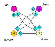
In legged locomotion there are actually four phases – leg up, leg forward, leg down and leg back. A simple elaboration on the half-centre model can generate this pattern.
- Load and Start the parameter file Multi-Phase Oscillator(v5-2). As previously, you will probably need to set a Slow down factor.
This shows a four phase progression which could drive a leg.
- Click Pause after you have observed a few cycles of the rhythm.
If you look at the network in the Setup View, you can see that there are actually 2 mutually inhibitory half-centres present, the diagonal pairs N1 and N3 (labelled up-down) and the diagonal pairs N2 and N4 (labelled forward-back). However, these are coupled in a ring of one-way inhibition, such that each element inhibits (and thus terminates the activity of) the neuron that was active in the preceding phase. This one-way inhibition is organized in a clockwise direction, and activity in the network thus progresses in an anti-clockwise direction (N4→ N3→ N2→ N1→ N4 etc.). (You can see this by watching the colours in the Setup view.)
In this 4-neuron network none of the synapses have to decrement in order to get oscillation. Looking at the activity in detail can explain why.
Pick a time when N1 has just started spiking.
- Place a vertical cursor on the first N1 spike in the cycle, so that you can clearly see what is happening at that time.
N2 was spiking, but it receives inhibition from N1, so it stops spiking and its membrane potential starts to hyperpolarize. N3 was already inhibited, and it too receives inhibition from N1 so it remains hyperpolarized. However, N4 is not being inhibited by N1 because there is no synaptic connection, and N2 and N3, which could inhibit it, are both themselves inhibited and so silent. So the N4 membrane potential starts to recover and depolarize (it was inhibited in the previous phase). Eventually, its membrane potential reaches threshold and it starts to spike. It then immediately inhibits N1, and the rhythm moves on to the next phase of the cycle.
And so it goes on …
- Click Continue to resume oscillations.
- While the simulation is running, check, and then uncheck the picrotoxin box in the Experimental Control panel.
The difference in response with removal of picrotoxin between this and the reciprocal inhibitory circuit described previously can be explained by the change in synaptic properties (decrementing vs non-decrementing) between the circuits.
Question: What would happen if one neuron in this circuit were damaged or destroyed? In a real experiment, this could potentially be achieved with dye-mediated laser photo-ablation (Miller & Selverston, 1979).
- With the model running, select the menu command Neuron: Zap. This pauses the simulation until you click on a neuron (your choice which). This “zaps” the neuron – it effectively destroys it and takes it out of the circuit just like laser photo-ablation . Observe what happens. Did it fit your prediction?
- Unlike in reality, we can resurrect a neuron with the Neuron: Un-Zap command. This means that you can un-kill your selected neuron, and kill another one. Trust me, this is a lot quicker and easier than doing real experiments!
[Optogenetics: In some experimental preparations you can achieve reversible inactivation of specific neurons if you can manipulate the cell to express a light-activated chloride channel. Switching a light on then massively inhibits that neuron (assuming it has a hyperpolarizing chloride reversal potential) and stops its activity, which is restored when the light is switched off.]
It is quite difficult to understand what is going on in this circuit, but if you think through the network carefully, you can figure out how this works. On the other hand, that is precisely the point of modelling – it would be a bold neuroscientist who would bet money (or their reputation) on exactly what the output of this circuit would be under different conditions, but by modelling we can find out!
Sensory Feedback
There is ample experimental evidence that central pattern generators really do exist – in many animals the nervous system can generate rhythms in the absence of sensory feedback. However, there is also ample evidence that sensory feedback normally plays an important role. Animals obviously have to adjust a locomotor rhythm in the event of unexpected external stimuli – if you trip up, you will take an extra rapid step to avoid falling on your nose. But also, most rhythms run faster in the intact animal with sensory feedback present than they do when the CNS is isolated from such feedback.
Sensory feedback may accelerate rhythms simply by providing additional general excitation to the nervous system. However, they can also act directly on the pattern generator itself.
- Load and Start the parameter file Sensory Feedback (v5-2).
In this circuit N1 and N2 at the top are a reciprocal-inhibitory half-centre oscillator like we saw earlier. They drive flexion and extension as labelled in the Setup view. Each half-centre activates a peripheral muscle (N3 and N6), and each muscle activates a peripheral sense organ (N4 and N5). These mediate negative feedback onto their half of the pattern generator. The delay of this feedback has been set to 200 ms, to account for the time taken for muscle contraction and axonal conduction.
The system generates 6 cycles of oscillation in the duration of the simulation.
- Apply the drug curare by checking the box in the Experimental Control panel.
With the current settingsMenu Options: Run on change and Results view Auto clear, this clears the screen and re-runs the experiment with the drug applied.
Curare (the famous South-American poison arrow drug) blocks nicotinic acetylcholine receptors and hence paralyses muscles and so disables the feedback. So in the presence of curare, the CPG oscillates at its intrinsic, free-running, frequency with no sensory feedback.
The oscillator now only generates slightly more than 4 cycles in the duration of the simulation. It is clearly running slower.
In this case, the cause of the frequency change is that the negative sensory feedback in the intact system is timed so as to truncate each burst of its half-centre driver, thus releasing the other half-centre early from its inhibition. This truncation allows the whole system to oscillate faster.
This is very much a “thought experiment” simulation. It illustrates one way in which sensory feedback could influence CPG frequency, but it is undoubtedly a massive simplification of the way real systems work.
Phase Resetting Tests
The frequency (or period) and phase are key characteristics of an oscillator, and if you do something experimentally that alters either of these, then you know that you have somehow affected the rhythm generation mechanism itself.
- Load and Start the parameter file Reset Test (v5-2).
Two neurons are visible and both oscillate. However, the program has been set up to hide any connections that might exist. This makes things a bit more realistic, since in a real experiment you cannot normally see connections between neurons (you are lucky if you can even see the neurons!).
So are both neurons endogenous bursters, or is it a network oscillator, or some sort of mixture?
Note that at the far right of the Results view, both neurons end the simulation run just at the completion of a spike burst.
- Set the amplitude of stimulus 1 to +0.5.
- Click Start without clearing the screen first.
The first part of the sweep is unchanged, but the stimulus induces a large burst of spikes in N1 and N2 (even though the stimulus was only applied to N1), and after that, things change. At times when the neuron was previously spiking it is silent, and when it was silent, it is spiking. In the new sweep the spikes “fill in the gaps” in the previous sweep.
- To see this more clearly, set the Highlight sweep to 1 in the Results view, and then change it to 2.
Note that while previously, with no stimulus, the sweep ended at the end of a spike burst in both neurons, it now ends just after the start of a spike burst in both neurons. This is because the stimulus forces the neurons to produce a burst of spikes earlier than they would have normally, and then after this early burst, the bursts continue at the same intervals that they had previously. The stimulus pulse has thus reset the phase of the rhythm, indicating the neuron 1 is part of the rhythm-generating circuit. The question now is, is N2 also part of the rhythm-generating circuit?
- Click Clear.
- Switch the stimulus to apply it to N2.
- Either drag the stimulus box in the Setup view and drop it on N2,
- or set the Target Neuron in the Experimental Control panel to 2.
- Click Start.
The stimulus now induces an early burst of spikes in N2 but not in N1. Furthermore, this does not reset the phase of the rhythm. To confirm this:
- Do not click Clear.
- Set the stimulus amplitude to 0.
- Click Start.
With the two sweeps superimposed, you can see the early burst in N2 produced by the stimulus, but you can see that this has no effect on the rhythm – the bursts continue on afterwards just as though there was no stimulus at all.
This tells us that N2 is a “follower” neuron that does not actually participate in generating the rhythm. It is simply driven by a rhythm that is generated elsewhere – which in this case must be N1, since there is nothing else.
To see the actual circuit:
- Click Connexions in the drop-down menu at the top of the main view.
- Note that there is a tick-mark beside the Hide connexions menu option.
- Click that option to de-select it and show connexions.
You can now see that N1 makes a non-spiking excitatory synapses onto N2. N1 is indeed an endogenous burster, and N2 is simply following the activity of N1 through its synaptic input. Anything you do to N2 has no effect on N1 because there is no synaptic connexion from N2 to N1.
Tadpole Swimming: A case study
Tadpoles may sound like rather obscure animals for a neuroscienist to study, but in fact the neural mechanism controlling swimming in hatchling tadpoles (charmingly known as polywigglesFrom old English poll = head (as in poll tax) and wiggle = wiggle! in Norfolk!) is one of the best understood vertebrate CPGs (Roberts, et al., 2010). At a behavioural level, swimming can be initiated by a brief sensory stimulus (touch) to one side of the body, and is driven by wiggling the tail in left-right alternating cycles at 10-25 Hz, with a wave that propagates from head to tail. The core mechanism depends on interactions between just two types of interneurons: descending interneurons (dINs) and commissural interneurons (cINs). These occur as separate populations on the left and right side of the animal, but the dINs on each side are coupled to each other, so that they excite each other and essentially act as a single unit. The dINs excite trunk (myotomal) motorneurons on their own side of the spinal cord, so if the left dINs spike, the tail bends to the left, and if the right dINs spike, the tail bends to the right.
DINs are glutamatergic neurons that arise in the hindbrain and rostral spinal cord. Because of their mutual excitation they develop a long-lasting NMDA-receptor mediated depolarization during swimming, and it is this depolarization that maintains swimming for episodes that can last from a few seconds to more than a minute. The dINs also drive the ipsilateralIpsilateral means on the same side, as opposed to contralateral which means on the opposite side. cINs through brief AMPA-receptor mediated EPSPs. The cINs are gylcinergic and feed inhibition back to the dINs, but on the other (contralateral) side of the spinal cord. It is thus the cINs that provide the reciprocal inhibition necessary to produce the alternating swimming rhythm. Unilateral lock-up is prevented by the cellular properties of the dINs, which each only spike once for a given depolarization. In order to spike again, there has to be an intervening hyperpolarization, which is provided by the cIN feedback. Thus during swimming the dIN spikes are triggered by rebound excitation from the IPSPs generated by the cINs.
The following simulations are based on parameters modified from Sautois et al., (2007). We will build up the circuit gradually, so that you can see the contribution of the components at each stage.
Basic dIN and cIN properties
- Load and Start the parameter file Tadpole dIN cIN.
There are two neurons, a single dIN and a single cIN, but there is no connection between them. Each receives stimuli (1 - 3), but these initially have 0 amplitude, so the traces are flat.
- With stimulus 1 selected, click the up arrow of the amplitude spin button in the Experimental Control panel and observe the effect of the long-duration stimulus in the dIN - initially it is a simple sub-threshold depolarization.
- Repeatedly click the up arrow until the amplitude reaches 0.1 nA.
The dIN starts to spike when the amplitude reaches 0.06 nA, but it just generates a single spike, even when the stimulus exceeds threshold. As you continue to increase the stimulus, the dIN produces some post-spike oscillations, but it does not generate more than just the single initial spike. This is a rather unusual property for a neuron, but it is characteristic of dINs in the tadpole.
- Select stimulus 2 (by clicking it in the list or clicking its box in the Setup view), and click the up arrow of the amplitude spin button to inject depolarizing current into the cIN.
- Repeatedly click the up arrow until the amplitude also reaches 0.1 nA.
The cIN has a slightly lower threshold than the dIN, and once threshold is exceeded it generates multiple spikes, which increase in frequency as the stimulus strength increases. This is a more normal neural response to stimulation. The cause of the difference lies in the kineticsIf you wish you can double-click a neuron to open its Properties dialog and then examine the voltage-dependent channels. But unless you're really interested you don't need to get into that level of detail if you just accept the properties at a functional level. of the voltage-dependent ion channels in the two neurons.
- Select stimulus 3 . Note that this stimulus is applied to both neurons.
- Click the down arrow of the amplitude spin button, to inject a brief pulse of negative current (-0.01 nA) into both the dIN and the cIN.
The dIN, which is depolarized but not spiking at the time of the negative pulse, responds by generating a small spike at the termination of the pulse. This is a case of rebound excitation as demonstrated earlier in the classic HH model, and has the same underlying cause: relief of inactivation of voltage-dependent sodium channels, and closure of open voltage-dependent potassium channels.
- Click the down arrow of the stimulus 3 amplitude spin button a few more times until the amplitude reaches -0.05 nA.
Note that increasing the hyperpolarization increases the size of the rebound dIN spike, and blocks spikes in the cIN.
Next we start to connect the neurons:
- Load and Start the parameter file Tadpole dIN cIN PIR.
As before, the upper neuron in the Setup view is a dIN, and it now makes an NMDA-type excitatory connection to itself (the blue diamond labelled c). This synapse represents the re-excitation of the whole population of dINs caused by the reciprocal synapses that they form with each other. The lower neuron is a cIN, and if it spikes, it will inhibit the dIN through its glycinergic synapse (the blue diamond labelled b).
Initially, the cIN is silent, but the dIN spikes in response to stimulus 1. The recurrent dIN excitation is visible as a long-lasting depolarization following the spike.
- Apply the drug AP5 (amino-5-phosphonopentanoic acid) by checking its box in the Experimental control panel. This is a selective antagonist of the NMDA receptor, and it abolishes the depolarization following the dIN spike.
- Remove the AP5, and click the up arrow of the amplitude spin button of stimulus 2. This stimulus makes the cIN spikeIn passing, note that the cIN spike is briefer than the dIN spike. The dIN spikes are in fact unusually broad for vertebrate spiking neurons., which in turn produces an IPSP in the middle of the self-induced depolarization of the dIN. The dIN generates a rebound spike as its membrane potential recovers following the IPSP.
- Apply the drug strychnine, which blocks glycine receptors. The IPSP disappears, as does the rebound dIN spike.
- Finally, remove the strychnine and re-apply AP5. The dIN only produces a rebound spike if the IPSP occurs during the activity-induced depolarization - the dIN does not spike on rebound from an IPSP occurring at resting potential.
The core swimming circuit
Now that we have seen the key properties of the individual dINs and cINs and how they interact with each other, we can build a minimalist CPG circuit.
- Load and Start the parameter file Tadpole Core CPG.
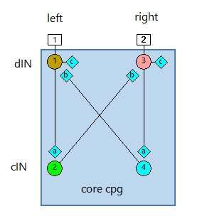
First look at the circuit in the Setup view. There are 4 neurons in total, comprised of a left-right pair of dINs (N1, N3 in the top row) and a left-right pair of cINs (N2, N4 in the bottom row). Each dIN excites itself through a long-lasting NMDA-type synapse (c), and its ipsilateral cIN through a brief (phasic) AMPA-type synapse (a). Each cIN inhibits its contralateral dIN through a phasic glycinergic synapse (b). Of course, each neuron in the model represents many neurons in the real animal, and the whole circuit is replicated many times along the length of the spine. So this is very much a simplified "concept model" of the real situation.
Now look at the Results view. Swimming is initiated by separate stimuli (bottom trace) applied to the left and right dINs, but once initiated it is self-sustaining. We will come back to the initiation later, but for now concentrate on swimming itself.
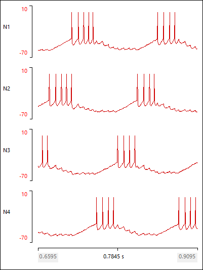
Swimming is characterised by alternating spikes in the left and right dINs (top and third traces, brown and magenta - each magenta spike occurs betweenOne easy way to check this is to drag the magenta trace up so that it overlays the brown trace. You can then see the relative timing. You can restore the position by resetting the top and bottom axes scales for the 3rd axis back to +40 and -70. two brown spikes). Since each dIN excites motorneurons on its side of the spine, this will generate side-to-side movement of the tail, resulting in swimming in the real animal. Note that the dIN spikes occur on top of a sustained depolarization caused by the recurrent excitation, which is interrupted periodically by IPSPs generated by the cINs (second and fourth traces, green and blue). In contrast, the cIN spikes result from brief EPSPs arising from the resting potential - there is no sustained depolarization.
- Select the Analyse: Timing menu command to display the Frequency etc vs Time dialog.
- Adjust the top Y axis to 50 Hz, and note that the dIN spike frequency stabilizes at about 25 Hz, which is within the range of normal swimming behaviour.
- Close the dialog.
Now examine the timing of the activity in the 4 neurons, ignoring the start of the simulation (because initiation is a tricky issue that we will return to).
- Click the expand timebase (
 ) button in the Results tool bar three times, and then click the Go to end button (
 ). You should now have a "zoomed in" view of the last part of the simulation.
 - Click the vertical cursor (
 ) in the Results toolbar, to give yourself a datum to see relative timing.
 - Drag the cursor to line up with the peak of the first visible dIN spike in the top trace.
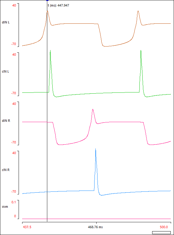
The left dIN (top trace, brown) activates the left cIN (second trace, green) with short latency, and this in turn generates a short-latency IPSP in the right dIN (third trace, magenta). It takes time for the right dIN to recover from this IPSP, but when it does, it generates a rebound spikes. This then generates a spike in the right cIN (fourth trace, blue), which feeds back to inhibit the original left dIN (back to the top trace). And so the sequence continues. The key element determining the cycle period in this circuit is the recovery time from the IPSP. This depends in part on the properties of the IPSP itself, but also on the voltage-dependent characteristics of the long-term EPSP in the dIN.
- Remove the vertical cursor by right-clicking anywhere in the Results view, and selecting Del all vert cursors from the context menu.
Spike-Triggered Display
A useful technique that can emphasise the timing and consistency of synaptic interactions is to use a spike-triggered display (see e.g. Fig 3c in Roberts et al., 2010).
In the Results view:
- Clear the screen.
- Select Spike triggered from the Trigger mode frame.
- Set the right-hand timebase axis to 50 ms.
- Uncheck the Auto clear box.
- Click Start.
Multiple sweeps are superimposed, each showing one cycle of swimming. The important point is that the sweeps are all aligned so that the membrane potential of the left dIN (specified as the trigger neuron, 1) crosses 0 (pre-defined as the synaptic trigger level in the neuron properties dialog) at exactly 5 ms (the specified pre-trigger delay) after the start of the sweep display.
Because the left dIN spikes (top trace, brown) are all aligned and the dINs drive the ipsilateral cINs with a fixed synaptic delay, the left cIN spikes (second trace, green) are also aligned. The left cIN spikes cause IPSPs in the right dINs (third trace, magenta), which are aligned, and these generate rebound spikes in the right dINs, which activate the right cINs (fourth trace, blue). And this leads to the next cycle.
The variability in the display is because the swim pattern takes a few cycles to "settle down" after initiation. You can see this by looking selectively at individual sweeps:
- Set the Highlight sweep to 1 and mentally note the display. Pay attention to the orange trace (the right dIN) - this is a good monitor of activity.
- Advance the Highlight sweep value by clicking the up arrow on the spin button until you reach sweep 10 (there are 25 in total).
You should see that the first few sweeps vary, but after about sweep 6 the pattern stabilizes, and subsequent sweeps are identical.
To get an overview of the "typical" pattern you can look at the average of the sweeps:
- Select the Analyse: Average menu command.
The Results view now shows each trace as the point-by-point average of all 25 sweeps. The raw sweeps are shown in grey, while the average is shown as a highlighted trace. The average spike peaks are smaller because of the variation in spike timing in the early sweeps, but the overall pattern of activity is very clear.
Swim initiation
In the simulation above, swimming is initiated by separate stimuli to the left and right dINs, but these stimuli have a 40 ms time delay between them (stimuli 1 and 2 occur at 25 and 65 ms respectively). This is a bit unrealistic. It is hard to image how a single sensory stimulus could drive the two sides with such a long delay between them - tadpoles are very small, and axonal conduction across the body could not take more than a few milliseconds.
What happens if the two sides are driven simultaneously?
- Reload the parameter file Tadpole Core CPG to get back to the starting conditions.
- Change the delay for stimulus 2 from 65 to 25 ms (the same as stimulus 1).
- Click Start.
The circuit still produces activity, but the two sides spike synchronously (left and right dINs spike together rather than in alternation), and the frequency is more than doubled. This would not produce an effective swimming behaviour. The cause of the synchronicity is that when the two sides are activated at exactly the same time, the crossed inhibition occurs immediately after each dIN spike, rather than with a half-cycle delay. However, this is a metastableLike a knife balanced on its edge - it will tend to fall one way or the other with any random perturbation. condition - if noise is added to the system, then sooner or later it collapses into the more stable pattern of left-right alternation.
- Load and Start the parameter file Tadpole Core CPG w Noise (you may want to set the Slow down factor > 0 to make the activity more easily visible).
The circuit is exactly the same as before, but random noise has been added to each neuron. The pattern (probably) starts in the high-frequency synchronous mode, but sooner or later it (probably) collapses into the alternating mode. You may need to run the simulation several times, since with random noise it is not possible to predict in advance when the switch will occur.
Surprisingly, synchronous activity does occasionally occur in the real animal (Li et al., 2014), but it has no known function and is probably a "mistake". It normally only lasts briefly, before relapsing into normal swimming. It is likely caused by the synchronous activity occupying a similar metastable state as seen in the simulation.
In the real animal it would not be satisfactory to rely on noise to perturb a metastable equilibrium, since the timing is unpredictable. To solve the swim initiation conundrum, we have to bring in another class of interneurons, the ascending interneurons (aINs). AINs are rhythmically active during swimming, but they inhibit ipsilateral neurons in the CPG - in particular, they inhibit the cINs.
- Load and Start the parameter file Tadpole Initiate (v5-2).
The Results view shows good swimming activity, but the Setup view shows that there is only one stimulus applied to the circuit to initiate swimming, so there can be no bilateral difference in stimulus timing.
The Setup view also shows that there are 3 new neurons in the circuit. N5 and N6 are aINs. They receive AMPA-receptor mediated EPSPs from their ipsilateral dIN (which is what makes them rhythmically active), and they make glycinergic inhibitory output to their ipsilateral cIN. N7 (at the top of the Setup view) is a left-hand sensory neuronThis neuron uses simplified integrate-and-fire spikes rather than the full HH formalism, since its only job is to generate PSPs in the neurons post-synaptic to it.. It makes bilateral excitatory input to both the dINs and the aINs. This is definitely an oversimplificationFor instance, there are other interneurons interposed between the sensory neurons and the cpg neurons. of the real circuit, but it conveys the essential features.
- Click the expand timebase () button in the Results tool bar three times to "zoom in" on the initiation stage of swimming.
- Activate a vertical cursor (click in the Results toolbar), to give yourself a datum to see relative timing.
- Align the cursor on the sensory neuron spike (bottom trace).
The key point with respect to swim initiation is that there is a delay in the sensory activation of the contralateral aIN. All synaptic delays in the simulation have been set to 1 ms, except the N7-to-N6 connection, which has a delay of 3 ms. The following sequence takes you through the consequences of this delay:
- On the left-hand side (ipsilateral to the stimulus), the aIN (trace, orange) spikes immediately following the stimulus. This left aIN spike is early enough to inhibit the cIN on that side (2nd trace, green), and prevent it from spiking.
- This means that the right dIN (4th trace, magenta) does not receive an IPSP immediately after its spike (as it did during synchronous activity above), and does not generate an immediate rebound spike.
- On the contralateral side, the extra 2 ms in the activation time of the right aIN (6th trace, dark green) means that the right cIN (5th trace, blue) can "escape" and is not inhibited. Note that the left and right cINs are activated at exactly the same time, but the left cIN receives the aIN IPSP before it spikes (which prevents it from spiking), while the right cIN does not receive the aIN IPSP until after it spikes.
- This means that the left dIN (1st trace, brown) does receive an IPSP immediately after its first spike, and its second spike therefore occurs early. However, after this one early double-frequency spike, the rest of the swim episode shows the normal alternating pattern.
This asymmetry in dIN activation essentially replicates the 40 ms relative delay in dIN activation used in the core circuit simulation to initiate swimming, but it does it using only a 2 ms difference in activation time between aINs on the left and right sides of the animal, which is within a plausible biological range.
Take-home message: The swimming rhythm in hatchling tadpoles is primarily driven by spikes in descending interneurons (dINs). These spikes activate commissural interneurons (cINs), which in turn inhibit contralateral dINs. The dIN spikes themselves result from post-inhibitory rebound from this contralateral inhibition, superimposed on an NMDA-receptor mediated background depolarization. The background depolarization is caused by mutual re-excitation between dINs.
Short-Term Motor Memory and the Sodium Pump
Tadpoles swim in episodes that can last from a few seconds to several minutes (although in the simulations above, they last indefinitely). In a real tadpole, an episode can be terminated abruptly by a mechanical stimulus to the cement gland on the head, such as a “nose bumpThe sensory input induced by the stimulus activates GABAergic neurons in the hindbrain, which in turn inhibit the spinal circuitry involved in generating the swimming rhythm.” collision with an obstacle (or even the under-meniscus of the water surface). However, even without such acute sensory inhibition, natural swimming frequency within an episode gradually slows, and eventually the episode self-terminates. If a second swim episode is induced by appropriate excitatory stimulation within a minute or so after the natural termination of the previous episode, the duration of the second episode can be substantially reduced. The shorter the gap between the episodes, the greater is the shortening effect. It thus appears that the spinal circuitry "remembers" its previous activity for a brief period, and this memory affects its subsequent output. This phenomenon has been termed short-term motor memory (STMM: Zhang & Sillar, 2012).
The mechanism underlying STMM in tadpoles is, at least in principle, surprisingly simple. At the termination of an episode of swimming, the membrane potential of most spinal neurons, including cINs, shows a small (5-10 mV) but significant period of extended hyperpolarization. This can last for up to a minute (similar to STMM), with the potential gradually returning back to its pre-swim resting level during this period. Thus, if the second swim episode is elicted during this ultra-slow after-hyperpolarization (usAHP), the duration of the second episode is reduced. If the gap between episodes is short, the usAHP amplitude induced by the first is still relatively large and the STMM effect is pronounced. If the gap is longer, the usAHP amplitude has decreased and the STMM effect is reduced. If the gap is sufficiently long that there has been full recovery from the usAHP, then there is no STMM, and the second episode duration is normal.
So the next question is, what causes the usAHP? This too has a quite simple explanation. During the swim episode the cINs spike repeatedly at up to 25 Hz, and during this period, there is a substantial inflow of sodium ions into the neuron, carried in part through the voltage-dependent sodium channels of the spike itself, and in part through the AMPA-receptor mediated EPSPs that drive the cIN spikes. The sudden influx of sodium overwhelms the constitutive sodium clearance mechanism (the standard Na/K ATPase: the “sodium pump”), so the intracellular sodium concentration starts to rise. This activates a specific alpha-3 sub-type of sodium pump which has a lower affinity for sodium and is normally silent, but is activated by high concentrations of intracellular sodium. This “dynamic” sodium pump, like the standard pump, is negatively electrogenicIt pumps 3 Na+ ions out for every 2 K+ ions it pumps in, leading to a net hyperpolarizing current. and it is this which causes the usAHP. As the excess sodium is cleared from the neuron, the dynamic pump activity declines, and thus so does the usAHP.
- Load and Start the parameter file Tadpole STMM.
A pair of stimuli is applied to the dINs to elicit an episodeNote the very slow timescale, so individual cycles within the episode merge on the screen to appear as a solid block. of swimming. Unlike in previous simulations, the episode self-terminates due to the development of the usAHP. [Note that there are other mechanisms that contribute to self-termination of swim episodes (e.g. Dale, 2002), but they are not implemented in this simulation.]
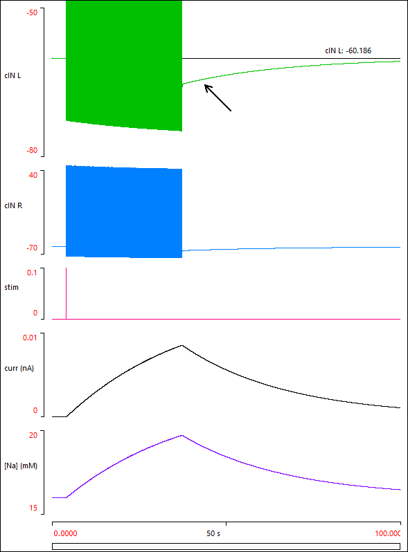
The top trace (green) shows activity in the left cIN during the episode. The vertical scale has been expanded to "zoom in" on the base membrane potential, to make the time course of the usAHP clearly visible. Before the episode the resting membrane potential is -60 mV, immediately after the episode it has hyperpolarized to about -65 mV (peak usAHP), and then it slowly recovers back to -60 mV over about a minute. The second trace (blue) shows the right cIN at a normal scale, so that the spikes are fully visible. The usAHP is identical in this neuron, but less obvious at this scale.
The episode terminates because the usAHP eventually causes the dIN-mediated EPSP in the (left) cIN to drop below threshold. This breaks the feedback loop, and terminates the episode.
The bottom trace (purple) shows the intracellular sodium concentration in the left cIN. It rises during the swimming episode, and then falls again after the episode, as the dynamic sodium pump restores the concentration to its resting level. The 4th trace (black) shows the hyperpolarizingThe pump current sign convention follows that of a normal ionic channel, so an upward deflection indicates an outward (hyperpolarizing) positive current. current generated by the dynamic pump, which mirrors the change in sodium concentration, and which is directly responsible for the usAHP.
Implementation details: The circuit is identical to that shown previously, but the voltage-dependent sodium channels and the AMPA receptors in the cINs have been set to have sodium as their carrierAMPA receptors are mixed cation channels, so the sodium component is set at 50% of the total current. ion. This is achieved through the relevant Properties dialogs. In addition, the cINs have a sodium concentration-dependent electrogenic sodium pump, which generates the usAHP. The dINs are unchanged from the previous simulations. (They do in fact have a putative usAHP, but this is masked by a hyperpolarization-activated current Ih (Picton et al., 2018) and so is ignored in this simulation.) Note that quantitative parameters determining sodium concentration and pump rate are heuristic - there is no physiological evidence for the values in this system .
- With stimulus 1 selected, click the Gauss selection for the stimulus. Repeat for stimulus 2.
- Click Start (no need to clear the results, because Auto clear is pre-selected).
The Gauss stimulus option has been set up to deliver two episode-initiating stimuli to the dINs, with the second occurring about 7 s after the termination of the first episode. The second pair of stimuli successfully initiate another swim episode, but the duration of this second episode is much shorter than that of the first. This is short-term motor memory!
- Select the Analyse: Timing menu command to open the Frequency etc. vs Time dialog.
- Set the top scale of the Y axis to 50 Hz.
The decline in cycle frequency within each episode, and the shorter duration of the second episode, are clearly visible.
- Close the dialog.
The cause of the reduced duration of the second episode is fairly obvious from the sodium pump current trace (black, fourth trace). At the time of the start of the second episode the pump current has only slightly declined from its peak level, and so as more sodium floods into the cell (purple, bottom trace) the pump current soon returns to the level that was sufficient to render the cIN EPSP sub-threshold, and thus to terminate the second episode.
- Change the Mean interval value for both stimuli from 40 to 60 s. This will delay the second swim-initiating stimulus.
- Click Start.
The gap between the end of the first episode and the start of the second is now longer and the dynamic pump has had more time to clear sodium from the cell, and so its current level is reduced. It therefore takes longer to return to the peak level that blocks the cIN EPSP, and the duration of the second episode is extended, although still considerably shorter than that of the first.
Take-home message: A dynamic sodium pump in cIN neurons generates an ultra-slow after hyperpolarization (usAHP) in response to the increase in intracellular sodium concentration that occurs during a swim episode. If a second episode is initiate before the usAHP has decremented to rest level, the duration of the second episode is reduced in a gap duration-dependent manner. This mediates a short-term motor memory (STMM).
Finally, it should be noted that there is increasing evidence that sodium pump-induced usAHPs are widespread in the nervous system of many animals. In some cases they may mediate STMM as in the tadpole, in others they may have different functions, such as protecting from excitotoxicity-inducing hyperactivity in hippocampal neurons (see Picton et al., 2017, for references).
Synchronization and Entrainment
People who study oscillators (particularly physicists) distinguish between synchronization and entrainment. Synchronization occurs when independently-rhythmic entities interact with each other bi-directionally to produce a coordinated system response. Entrainment is when the interaction is one-way. Thus our circadian clock is entrained by the external day-night light cycle (our internal biological clock does not affect the rotation of the earth!), but the multiple neural oscillators in the suprachiasmatic nucleus that maintain our clock synchronize each other by mutual interaction.
Entrainment
- Load and Start the parameter file Entrainment.
The single neuron shows an endogenous rhythm. It does not have full H-H spikes, but that doesn’t matter for our purpose, what matters is that it oscillates at a fixed frequency which is determined by its intrinsic properties.
- Without clearing the screen, set the Amplitude of Pulse 1 to 0.04 (a single click on the up arrow of the spin button should do it).
- Click Start.
A repetitive stimulus now occurs with a frequency which is slightly faster than the endogenous rhythm. The stimulus continuously “pulls” the oscillation forward, so that on each cycle it occurs slightly earlier than its endogenous frequency. This is an example of entrainment, and the stimulus could be called a forcing stimulus.
- Use the Highlight sweep facility in the Results view to look at each sweep in turn to make sure you understand what is happening.
- Select the Analyse: Timing menu command to open the Frequency etc vs Time dialog, and move the dialog so that it does not obscure the Results.
Note that a red horizontal cursor has appeared in the Results view. This acts as a threshold for spike detection.
With the default settings, the dialog displays the instantaneous frequency of spikes in the Results view. A "spikeIt doesn't have to be an actual spike. Any oscillation that goes above threshold and then drops below threshold is regarded as a spike." is regarded as occurring during a time period in which the membrane potential goes above the red cursor. Instantaneous frequency is the reciprocal of the time interval between the onset of spikes, so there is one fewer frequency value than there are spikes in the display. Various other analysis options are available within the dialog, but they are not used in this activity.
- The default threshold value is suitable for this analysis, but if it were not you could adust its position by changing the Threshold value within the dialog, or simply by dragging the red cursor to a new location in the Results view.
The row of dots across the dialog screen shows the instantaneous frequency of the oscillation.
- Check the Autoscale Y box near the bottom of the dialog to get a more accurate view of the frequency.
- Hover the mouse over a dot, and read the frequency as the Y value displayed to the left of the graph near the bottom of the dialog. It should be about 1.6 Hz. (You could also just look at the Y axis scales.)
This is the frequency of the oscillations in sweep 1 (the sweep ID is shown at the top-left of the dialog), which is the endogenous rhythm without the forcing stimulus.
- Check the Concat[enate] sweeps box near the top of the dialog.
Both sweeps are now displayed in sequence in the frequency graph. Note that in the second sweep, on the right side of the dialog graph, the frequency increases to 1.8 Hz. This is the result of the forcing stimulus entraining the rhythm to a higher frequency.
How far can a forcing stimulus push a natural rhythm to change its endogenous frequency? The answer depends entirely on the properties of the stimulus and of the mechanism generating the natural rhythm. But we can explore this a bit in the current simulation.
- Click Clear in the main Results view. (The frequency graph now indicates that there are no data for analysis.)
- Change the sweep duration to 20 s by editing the right-hand x axis scale. This will give us more time in which to establish a rhythm.
- Successively set the stimulus amplitude to 0 (zero), 0.04 and then 0.03, clicking Start after each change. Do not clear the screen between runs.
The first two sweeps exactly repeat the previous experiment, but the third sweep attempts entrainment with a weaker forcing stimulus. The frequency graph should now look like this:
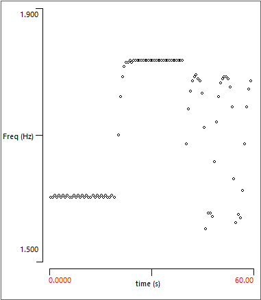
The weaker stimulus attempts to increase the rhythm frequency, but periodically fails. This can be seen more clearly by looking at the individual sweeps.
- Uncheck the Concatenate sweeps box in the frequency dialog.
- View Sweeps 1, 2 and 3 successively.
To see what is actually happening we need to zoom on the relevant section in the Results view.
- Set the start time (left-hand timebase axis) to 5 s and the end time (right-hand timebase axis) to 9 s.
- Switch the Highlight sweep between 2 (with the 0.04 nA stimulus) and 3 (with the 0.03 nA stimulus).
You can see that with the stronger stimulus (sweep 2) every cycle of the rhythm is entrained: there are 7 stimulus pulses visible in the display and 7 spikes, so each stimulus is followed by a spike. However, with slightly weaker stimulus (sweep 3) there are still 7 stimulus pulses, but only 6 spikes. The rhythm "skips a beat" on the 4th visible stimulus.
Take-home message: A periodic forcing stimulus can entrain an endogenous neural oscillator to a different frequency, but only within certain range.
Synchronization
Most real oscillator circuits involve a pool of neurons with quite similar properties, rather than just single neurons. This makes the circuit more robust, since individual neurons in the pool can be damaged or destroyed without seriously impairing the circuit as a whole. However, there has to be some way of synchronizing the neurons, and this is typically accomplished by electrical coupling between local neighbours. This enables a neuron which is oscillating too rapidly to be “pulled back” by current drain into its more restrained neighbours, while one which is going too slowly will be helped along. This process is called synchronization.
WARNING: The following simulation involves flashing multi-coloured lights. If you could be adversely affected by this sort of visual stimulus, you should use Neuron: Colours: Edit colour map to change the map to monochrome, or remove the colours entirely by unchecking Colour from voltage.
- Load and Start the parameter file Synchronization.
There is a 10 x 10 matrix of neurons, each of which is a non-spiking endogenous burster. The bursters have identical properties and they start off synchronized, but each has a substantial amount of membrane noise which will randomly perturb its rhythm. In the Setup view the neurons are colour-coded by their membrane potentials, and 4 neurons from the circuit are shown in detail in the Results view (the arrangement of 2 per axis is just to aid comparison).
- After admiring the pretty colours for a few moments, click Pause while you read on.
Each neuron is connected to its neighbours by electrical synapses. For clarity these have been hidden, but they can be revealed by deselecting the Connexions: Hide connexions menu option. BUT, in the default configuration as loaded, all the electrical synapses are blocked by the drug NEM (n-ethylmaleimide, a gap-junction blocker).
Because the electrical synapses are blocked, each neuron free-runs at its own intrinsic rhythm, and due to the random noise, they rapidly desynchronize.
- Click Continue to do just that.
- While the simulation continues to run, uncheck the NEM box in the Experimental Control panel.
This unblocks the electrical synapses, and the neurons rapidly synchronizeI was once lucky enough to see synchronized firefly flashing in the North Georgia mountains while on a family holiday. The similarity in visual appearance to the output of this simulation was striking, and the underlying mechanism of nearest-neighbour coupling is probably similar.. As soon as one neuron enters its depolarized phase, it “pulls” the others along after it, and a wave of depolarization sweeps across the whole network. Over time, the pattern of this wave can change, since the membrane noise means that it will not always be the same neuron that takes the lead role.
- Check and uncheck the NEM box a few times, and observe synchronization and de-synchronization.
- When you have seen enough, click Stop, and Clear the Results view display.
Spike vs Time mode
An alternative visualization can be achieved in the Spike vs Time mode.
- Select Spike vs Time in the Display mode group of the Results view.
- Click Start.
- If you want to speed things up, de-select the Neuron: Colours: Colours from voltage menu option (you may now need to set a non-zero Slow down factor).
- As the simulation progresses, check and uncheck the NEM box in the Drugs group of the Setup view to see the network move in and out of synchronization.
Metachronal Rhythm
In the previous simulation, all the oscillators had the same intrinsic frequency. However, this does not have to be the case.
- Load and Start the parameter file Metachronal Rhythm.
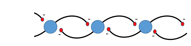
We have 5 neurons linearly coupled by electrical synapses into a nearest-neighbour chain, although as before, the synapses are initially blocked by NEM.
Each neuron is an oscillator, and can be thought of as representing the segmental CPG in a chain of ganglia such as might control, for instance, the legs of a centipede. The CPGs are not identical. The intrinsic frequency follows a segmental gradient, with N5 (the most posterior) being the fastest, and each segmental homolog being slower as they ascend rostrally in the chain. With the coupling blocked, each CPG free-runs at its intrinsic frequency.
- Watch the pattern of activation by observing the colour changes of the neurons in the Setup view.
After a short while, the coordination appears chaotic. Each neuron is oscillating at its own frequency, and the peaks drift past each other as the simulation progresses, producing an apparently random pattern of colour changes in the chain of neurons.
- Uncheck the NEM box in the Experimental Control panel.
After a few cycles, the CPGs now become synchronized. However, N5 always leads the rhythm, with the other segments following in sequence. Thus a metachronal rhythm is generated, in which a wave of excitation sweeps rostrally through the chain.
- While the simulation continues to run, select the Neuron: Zap menu option (the simulation then stops), and click on the central neuron N3 (the simulation restarts). This kills that neuron.
With the central oscillator removed from the circuit, the two ends now oscillate independently. The posterior end oscillates at relatively high frequency, driven by N5 as its pacemaker. The anterior end oscillates more slowly, with N2 acting as its pacemaker.
- You can use the Neuron: Un-zap facility to restore N3 to the circuit, and the faster rhythm now resumes throughout.
This very simple model uses just one of the many mechanisms that can produce a metachronal rhythm. However, it can generate testable hypotheses. It predicts that if you remove the central oscillator, perhaps surgically, or perhaps, more reversibly, by pharmacological intervention, the two ends will continue to produce coordinated oscillations, but at different frequencies. If you did that in a real system and found, for instance, that the back end continued to oscillate but the front end shut down, then this means that your system must be using a different mechanism to this model.
Stochastic Resonance: Noise Matters
Noise, in a signal processing context, refers to random fluctuations in a signal which do not have any information content relevant to the signal itself. Noise is usually thought of as a bad thing because it corrupts the signal - the receiver has no way of knowing which fluctuations in a signal are noise, and which are the information of interest. However, in some contexts, noise can actually be a good thing. In particular, in sensory systems, noise can enhance the sensitivity of the receiver to small signals through a process known as stochastic resonanceStochastic resonance theory was originally developed specifically for oscillating signals, but the term is now generally taken to include any situation in which noise enhances the performance of a non-linear signal processing system (McDonnel & Abbot, 2009). .
- Load the parameter file Stochastic Resonance.
- Check the Spike frequency graph box in the Display mode group of the Results view to open the Spike Frequency graph, and move its window to a convenient location. It is dockable, but there is no need to dock it anywhere unless you want to.
- This graph will show the average spike frequency in the two neurons, calculated after each simulation run. At the moment it is empty, because there has not been a run.
- Click Start.
The Setup shows two spiking sensory neurons (N1 and N2), receiving an identical stimulus input. The two sensory neurons are themselves identical, except that N2 has added noiseThe noise is generated by random current fluctuations following an Ornstein-Uhlenbeck distribution. This is a good approximation to noise generated by the random opening and closing of ion channels (Linaro et al., 2011). . The default stimulus amplitude is quite small (0.08). This generates a voltage response in N1 which is definitely below threshold, so N1 does not spike. It is also very unlikely that N2 spikes (unless the noise takes an exceptionally positive random value), so the stimulus is undetected by either sensory neuron.
- Click the up arrow on the stimulus amplitude in the Experimental Control panel to increase it slightly.
The Options: Run on change menu toggle has been pre-selected, so a new simulation runs when you change the stimulus amplitude. However, the stimulus is still quite small and it is unlikely to generate spikes in the sensory neurons (it certainly won’t in N1, it probably won’t in N2). Note that the purple bars in the frequency graph are both at or close to zero.
- Repeatedly click the up arrow on the stimulus amplitude until it reaches a value of 0.15, observing the traces in the Results view and the bars in the frequency graph, at each change.
As the stimulus amplitude increases, you should start to see occasional spikes in N2, which is the sensory neuron with added noise. The frequency of these spikes increases as the stimulus strength increases (note the N2 purple bar rises higher in the frequency graph). However, N1 remains silent even though it receives the same input.
Remember that N1 and N2 are identical apart from the noise, and so have exactly the same spike threshold. However, as the membrane potential in N2 gets close to threshold, the added noise occasionally lifts it above threshold, hence the spikes. N1 remains silent because without noise its threshold is never reached for these stimuli.
- Click the up arrow on the stimulus amplitude once, to take it to a value of 0.16.
The stimulus now finally crosses threshold in N1, which consequently generates spikes. However, the spike frequency in N1 immediately jumps to about 30 Hz – there is no graded low-frequency response like there was in N2.
- Click the up arrow on the stimulus amplitude twice more until it reaches a value of 0.18, observing the traces in the Results view and the bars in the frequency graph, at each change.
Both neurons now respond with approximately the same increasing spike frequency as the stimulus strength increases. Thus the noise has not reduced the coding capability of N2 relative to N1 in terms of the average spike frequency above N1 threshold, although the fine-timing capability is reduced due to the increased uncertainty in the exact moment at which threshold is crossed.
Take-home message: The noise increases the sensitivity of N2, so that it can respond to weaker stimuli than N1, even though they both have the same absolute spike threshold. Furthermore, the noise increases the dynamic range of N2, so that it is able to code the weaker stimuli with lower frequency spikes.
A key requirement for the occurrence of stochastic resonance is that the detecting system should be non-linear. The sensory neurons are highly non-linear because they generate spikes. When the input signal is below threshold they have zero output, when it is above threshold they generate spikes in which the input amplitude is coded by the output frequency. It is this non-linearity that causes noise to benefit signal detection. (If the neurons were non-spiking and their output was mediated by non-spiking synapses, then the noise would simply contaminate the output and be of no benefit whatsoever.) Of course, even in a non-linear system there is a limit to the benefit – if there is too much noise the signal will just become lost in the noise. In fact, for time-varying signals there is usually a single optimum noise level, which is why “resonance” is part of the name originally coined for the process.
Finally, it is worth pointing out that some level of noise is absolutely inevitable in any biological system, so all spiking sensory neurons will benefit from stochastic resonance to some extent. In man-made systems, engineers sometimes add noise specifically to optimizeThis is the principle that underlies dithering in commercial analogue-to-digital conversion processes. stochastic resonance, but I am not aware of any evidence for specific biological adaptations tuning the level of intrinsicIt has, however, been shown that adding noise to an external stimulus can enhance its detection through stochastic resonance (e.g. Levin & Miller, 1996). noise in sensory neurons to enhance their detection capability.
Lateral Inhibition
From an evolutionary perspective, paying attention to changes in the environment is probably more important than focussing attention on things that just carry on without change. The change can be something in time – the sudden noise that alerts you to the presence of danger, or in space – the visual line that demarcates the edge of a narrow path with a steep drop on one side. So it is not surprising that the nervous system is especially tuned to detect such changes.
One well-known mechanism for emphasising edges in a spatial field is lateral inhibition. This occurs in spatially-mapped senses such as the visual system, and it refers to the ability of a stimulated neuron to reduce the activity of neurons on either side of it.
- Load the parameter file Edge detector. (If you are using v5-2 the file Lateral inhibition 1D shows a similar effect.)
This is a concept simulation loosely based on the vertebrate retina. The top row is an array of spatially-mapped non-spiking receptors (or bipolar on-cells in the retina). Each neuron in the row inhibits those on either side of it through a non-spiking chemical synapse, thus mediating lateral inhibition. (The connections have been hidden for clarity, but can be revealed by deselecting the Connexions: Hide all connexions menu option.) The middle part of the array (N10 - N20) will receive a brief stimulus delivered through the square boxes when you run the experiment.
The lower row is an array of spiking interneurons (perhaps ganglion cells in the retina). Each interneuron is activated by its partner receptor in the row above through a non-spiking excitatory chemical synapse. The interneurons have some added membrane noise to enhance their sensitivity through stochastic resonance.
- Click Start.
The Results view shows activity in the receptor layer, but the Display mode has been set to Voltage vs Neuron. This means that the X-axis represents the individual neurons in the receptor array (N1 - N30), and the Y axis represents the membrane potential of each of those neurons. The whole display evolves over time, before stabilizing, at which point dots are drawn to show the potential of each neuron.
The response shows the clear edge-enhancement produced by lateral inhibition. If you hover over the two "cat's ear" peaks, the status bar shows that they are generated by N10 and N20, which are the two receptors just on the inside edge of the stimulus, while the adjacent troughs are generated by N9 and N21, which are just on the outside edge. The network thus differentially amplifies the response at the transition from unstimulated to stimulated receptors, compared to the stable conditions within the “body” of the stimulus, although there is still a clear difference in activity level in that region too.
Task: Think through how lateral inhibition produces the edge-enhancement that the simulation demonstrates. Explain it to a friend!
- Check the picrotoxin box in the Experimental control panel to block the lateral inhibition.
- Click Start.
- Use the Results Highlight sweep facility to look at the two sweeps in turn.
With the picrotoxin applied, the receptor array response is simply proportional to the strength of the stimulus – there is no edge-enhancement.
It is worth noting that lateral inhibition supresses the overall activity level compared to what it is without inhibition, and also reduces the difference in activity between the unstimulated response and the response in the “body” of the stimulus. However, the enhancement in the difference seen at the edge seems to be a worthwhile trade-off, given that lateral inhibition has been found in many sensory processing systems in many animals.
What happens in the spiking interneuron layer?
- Uncheck the picrotoxin box to restore lateral inhibition.
- Clear the Results.
- Select Spike vs Time in the Display mode group.
- Click Start.
The Result view now shows a raster plot of the spikes in the interneuron layer (N31 - N60), with each dot representing a spike.
It is very clear that N40 and N50 have a strongly enhanced spike rate during the stimulus. These are the interneurons that receive their input from the receptors just on the inside edge of the stimulus. The interneuron within the "body" of the stimulus spike occasionally, but at a much lower rate than those just inside the edge.
- Repeat the picrotoxin experiment to block lateral inhibition, and note that all interneurones within the stimulated region now have a high uniform spike rate.
To see the membrane potential responses of individual neurons:
- Uncheck the picrotoxin box to restore lateral inhibition.
- Clear the Results.
- Select Neuron vs Time in the Display mode group.
- Click Start.
The Results view shows the activity of a receptor and its paired interneuron outside of the stimulus (N5, N35; top two traces), just on the inside edge of the stimulus (N10, N40; middle two traces) and within the body of the stimulus (N15, N45; bottom two traces). Note that the spike responses will be variable due to the membrane noise, particularly in N45 which is close to threshold during the stimulus.
Take-home message: Lateral inhibition increases the perceived contrast at the edge of a spatially-mapped stimulus.
Pre-Synaptic Inhibition
One advantage of chemical synapses for communication between neurons is that they can be highly plastic - the strength of the connection can often be modulated, both on a long-term basis (e.g. long-term potentiation; LTP), and also on a moment-by-moment basis. One of the key mechanisms underlying the latter is pre-synaptic inhibition.
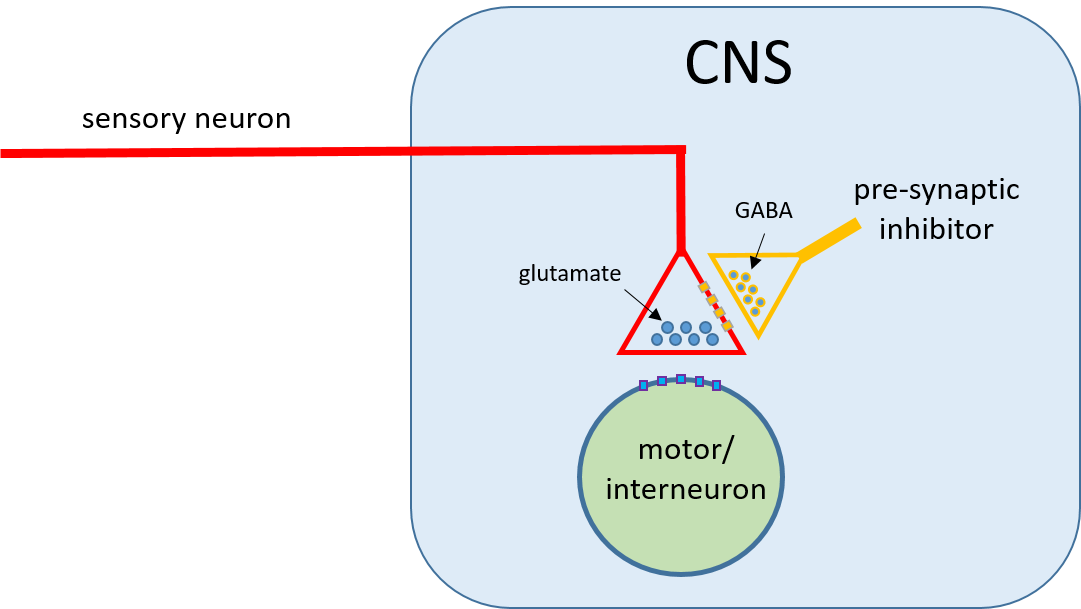
Standard post-synaptic inhibition is a familiar phenomenon - IPSPs impinge on a neuron and counteract the effect of any EPSPs occurring in the same neuron. Pre-synaptic inhibition is different - it occurs when an inhibitory neuron targets the release terminals of the excitatory pre-synaptic neurons that are delivering the EPSPs to the post-synaptic neuron, and prevents or reduces the release of transmitter. Pre-synaptic inhibition thus directly reduces the size of message impinging on the post-synaptic neuron, rather than merely counteracting its effects after it has already arrived.
Pre-synaptic inhibition is well established as a key mechanism for gating the flow of sensory information into the CNS. It would be quite difficult to stop a sensory neuron from actually responding to a peripheral sensory stimulus - this might require sending an inhibitory axon all the way to the periphery and inhibiting the sensory neuron at its transduction site. Post-synaptic inhibition could prevent a neuron from responding to sensory input, but it would also prevent it responding to any other input arriving at the same time. If an animal needs to block sensory input from a specific source but leave it responsive to other inputs, the answerThis is, of course, a totally post hoc argument - evolution often comes up with solutions to problems that do not seem to be the most efficient way of doing things. is to allow the sensory neuron to respond as normal, but to stop it from making output in the CNS, and thus prevent it from having any effect.
Primary Afferent Depolarization (PAD)
Pre-synaptic inhibition of afferent neurons in the vertebrate spinal cord is mediated by the release of GABA from inhibitory interneurons, which activates GABAA receptors in the afferent terminals. This leads to an increase in chloride conductance in the terminals, and a consequent IPSP. However, there is an unusually high concentration of Cl- within the terminal itself (due to the sodium-potassium-chloride co-transporter NKCC1), and so the equilibrium potential for Cl- is depolarized relative to resting potential. The IPSP is therefore depolarizing, as discussed previously in the Synapse part of the tutorial. This is called primary afferent depolarization (PAD) (Engelman & MacDermott, 2004).
Depolarizing inhibition is highly counter-intuitive at first sight, and yet it is ubiquitous in sensory gating, and quite common elsewhere too. So how does it work, and what are its advantages?
- Load and Start the parameter file Pre-Synaptic Inhibition (v5-2).
The Setup view shows a sensory (afferent) axon snaking its way into the spinal cord. The axon is simulated as a compartmental model, with each segment implementing HH-type spikes and connected to its neighbours by electrical synapses (for simplicity, these electrical synapses are hidden in the Setup view). A spike is initiated in the peripheral segment (N1, top-left in the Setup view, red) by sensory stimulus 1. The peripheral spike is shown in the Results view top axis as the red trace. The spike propagates along the axon into the CNS, where after a short delay it arrives at the terminal output segment (N21 in the Setup view, green; Results view top axis green trace).
To make this clear:
- Click Clear in the Results view.
- Select the Neuron: Colours: Colour from Voltage menu command.
- Click Start.
You should see the spike propagating in the axon as a series of colour changes.
- Go back to the normal display by reversing the steps above.
Within the CNS the sensory neuron makes an excitatory synaptic connection to a post-synaptic neuron (N22, blue; this could be a motorneuron or an interneuron). The EPSPTo make the EPSP sensitive to the shape of the pre-synaptic spike, it is generated by a non-spiking synapse with a high threshold for transmitter release. is visible in the Results view 3rd axis (blue trace). For clarity, N22 has been made a non-spiking neuron, but the EPSP is quite large and could well elicit a spike if the neuron were capable of generating one.
The last twoTwo segments are inhibited purely for simulation convenience - it was easier to demonstrate the phenomenon when two rather than one segment received the inhibition. I expect that with suitable adjustment of parameters a similar effect could be achieved by inhibiting just one segment, but since the segment boundaries are purely an artefact of the compartmental model methodology, this did not seem worth the effort. segments of the afferent axon receive pre-synaptic inhibition from an interneuron (N23, orange), but this is not activated in the default situation (no spike is visible in the lower axes of the Results view), so there is no inhibition.
- Set the amplitude of stimulus 2 to 8 nA in the Experimental Control panel to the left of the Setup view (you can do this by just clicking the up-arrow of the spin button).
- Run on change is pre-selected in the Options menu, so a new simulation runs, with traces superimposed in the Results view.
Several changes are visible:
- There is a spikeThis neuron uses simplified integrate-and-fire spikes rather than the full HH formalism, since its only job is to generate the IPSPs in the afferent terminal. in the pre-synaptic inhibitor neuron (orange trace: this is an integrate-and-fire neuron, so the spike is just shown as a vertical line), which is timed to occur just before the afferent spike arrives in the terminal segment of the afferent axon.
- A depolarizing potential is visible in the membrane potential of the terminal segment (green trace ) which starts before the spike arrives in that segment. This is the PAD generated by the pre-synaptic inhibitor.
- The afferent spike in the terminal segment is reduced in amplitude and duration compared to the spike without PAD.
- The EPSP in the receiving neuron (blue trace) is considerably reduced in amplitude - this is the result of the PAD-induced pre-synaptic inhibition.
- Use the Highlight sweep facility in the Results view Trigger mode group to switch between sweeps 1 and 2, to make sure that you understand the difference between the two.
Inhibition Mechanism
Why does the PAD generate inhibition? This is still a matter of some debate, but there are generally thought to be 2 effects at play.
- Shunting: The increased chloride conductance in the afferent terminal will act as a current shunt, which increases the leak of the spike-induced depolarizing current, and hence reduces spike amplitude. However, this would also occur with a hyperpolarizing IPSP, so it does not explain why depolarization is so common.
- Sodium inactivation / potassium activation: The depolarization starts to inactivate voltage-dependent sodium channels and activate voltage-dependent potassium channels just before the afferent spike invades the terminal region. This will reduce the peak spike amplitude and duration.
Either mechanism would reduce the activation of voltage-dependent calcium channels in the pre-synaptic terminal and hence the inflow of calcium, thus reducing transmitter release.
At this stage you should have 2 sweeps visible on the screen, the first showing the blue EPSP without pre-synaptic inhibition, the second showing it with the inhibition. (If you have cleared the screen, repeat the experiments above to get back to this stage.)
- Select the Synapses: Spiking Chemical menu command to open the Spiking Chemical Synapse Type dialog. This is non-modal, so you can keep it open while running simulations.
If possible, move the dialog box so that it does not obscure the main window.- Select synapse type b: pre-synaptic inhibition in the Type list.
- Note that the equilibrium potential is -61 mV, which is depolarized relative to the resting membrane potential of the post-synaptic neuron (the afferent neuron), which is -70 mV, hence the depolarizing nature of the IPSP.
- Change the equilibrium potential to -70 mV.
- This is the same value as the resting potential, so it should generate a flat (silent) IPSP, with no PAD, and consequently no pre-inactivation of the terminal sodium channels. Any inhibition would have to be a consequence of shunting.
A third simulation runs, but this time there is no PAD (the green trace is indeed flat until the spike takes off). Remember that the inhibitory synapse is still being activated, and therefore there is still a GABA-induced increase in chloride conductance, but there is no voltage change in the afferent terminal. So the shunting effect (1 in the list above) is still present, but there is no effect on the voltage-dependent channels (2 in the list above).
This generates an EPSP in N22 (blue trace) that is smaller than the full-sized EPSP (sweep 1), so there is some inhibition, but larger than the EPSP generated with PAD (sweep 2), so the inhibition is not as effective. The pre-synaptic spike height is also intermediate between the other two situations.
- To help keep clear which result goes with which condition, highlight each sweep in turn by using the Highlight sweep facility in the Trigger mode group of the Results view.
Take-home message: Shunting alone produces some degree of pre-synaptic inhibition, but the inhibition achieved with PAD in combination with shunting is considerably more effective than that generated by shunting alone. [But note that this is a concept simulation and the parameters are not derived from experimental data, so the balance may vary in different real preparations.]
Question: What happens if you generate a hyperpolarizing IPSP?
-
- Set the equilibrium potential to -80 mV, which is below the resting potential.
- When the simulation runs, note that the afferent terminal spike in the green trace is now preceded by a hyperpolarizing potential.
There is now hardly any inhibition - the EPSP is almost the same size as the full-sized EPSP without inhibition. It appears that pre-synaptic hyperpolarization actually works against producing post-synaptic inhibition, presumably by relieving some of the sodium inactivation and potassium activation that occurs naturally at the resting membrane potential (see the Rebound Excitation tutorial).
Antidromic Spikes and the DRR
One of the weird consequences of PAD is that sometimes the depolarization can be enough to generate spikes in the sensory neuron, without any sensory stimulation occurring!
- ReloadThe easiest way to reload a parameter file is to select it from the first entry in the File: MRU (most recently used) list below the Notes command. the parameter file Pre-Synaptic Inhibition to get back to the starting condition.
- Set the amplitude of stimulus 2 to 8 nA to turn on pre-synaptic inhibition and PAD.
- Set the amplitude of stimulus1 to 0 nA to turn off the sensory stimulus.
- Click Clear, and then Start, to get a single simulation run.
There is no initial spike in the periphery of the afferent (red trace) because you have turned off the sensory stimulus (1), but the central inhibitory interneuron is still stimulated (2) and so the PAD occurs as a visible depolarization of the afferent central terminal (green trace).
- Re-open the Spiking Chemical Synapse Type dialog (select the Synapses: Spiking Chemical menu command).
- Set the equilibrium potential of the type b: pre-synaptic inhibition synapse to -60 mV, i.e. just slightly more depolarized than the default value of -61 mV.
- The simulation should run when you make the change.
- Click OK to close the dialog box.
The PAD is now slightly larger, and the depolarization is sufficient to generate a spike in the central terminal of the afferent (green trace). This antidromicIt is well known that under experimental conditions axons can propagate spikes in either direction. Spikes that travel in the normal direction are called orthodromic spikes, while spikes that travel in the opposite direction to normal are called antidromic spikes. spike propagates backwards down the axon, out to the periphery, but it also generates an EPSP in the post-synaptic neuron.
One might think that generating extra spikes in afferents would be the precise opposite of what was wanted to achieve inhibition. However, the PAD-generated spikes in the central region are of reduced amplitudeThe chloride equilibrium potential in a real sensory neuron may be above threshold, but it is always considerably below the sodium equilibrium potential. This means that the increased chloride conductance will tend to counteract the increased sodium conductance that normally determines peak spike amplitude., just like orthodromic spikes affected by PAD, so the EPSPs (blue trace) are also reduced compared to those generated by orthodromic spikes without pre-synaptic inhibition. So although there is some extra excitation, it may not have much effectAs stated before, this simulation is not based on quantitative data. It would be quite easy to change the simulation parameters so that pre-synaptic inhibition eliminated the EPSP entirely, but for demonstration purposes the phenomenon is clearer if some residual excitation is allowed to remain. on the post-synaptic neuron. Also, the antidromic spikes will collide with any orthodromic spikes coming up the same axon at that time, and prevent them from reaching the CNS, so this may actually contribute to inhibition (although the probability of such collision is likely to be quite small).
Antidromic spike generation as a result of PAD is quite common in real preparations because the chloride equilibrium potential in vertebrate sensory neurons is often above their spike threshold. One situation that can generate antidromic sensory spikes is massive sensory stimulation, such as that caused by the pain response to damaged tissue. The resulting PAD can be so large that it causes a volly of antidromic sensory spikes known as a dorsal root reflex (DRR). There is some evidence that this antidromic discharge in nociceptors may cause release of peptides from the peripheral afferent endings, which may in turn exacerbate inflammation of damaged tissue. There is thus the possibility of a pathogenicOf course, the inflamation may increase a behavioural "guarding response" that helps protect against further damage, and may even have beneficial anti-bacterial effects. We all hate pain, but sometimes it may be good for us! positive feedback loop (Lin et al., 1999).
The Jeffress Model for Auditory Localization
Many animals, including ourselves, are remarkably good at localizing where a sound comes from, but the overall champion is probably the owl (reviewed in Sillar et al., 2016, chapter 3). These birds can not only accurately determine the spatial origin of the faint rustle of a mouse crossing the floor, they can do it in complete darkness!
For horizontal (azimuth) localization, the owl uses the difference in the time of arrival of sound at its two ears. If the origin is straight ahead (or behind) the sound will arrive at the left and right ear simultaneously. If the sound comes from the right, it will get to the right ear first, and if it comes from the left, it will get to the left ear first. However, owls have quite small heads and sound travels rapidly, so the interaural time difference (ITD) is only in the order of microseconds. How can the nervous system measure time differences which are that small?
The Jeffress model (Jeffress, 1948) describes a neurocomputational mechanism for measuring such very small time differences. It was originally completely hypothetical, but there is now strong evidence that a Jeffress-like mechanism operates in the nucleus laminaris in birds (Carr and Konishi, 1988), and may also operate in the medial nucleus of the superior olivary complex in mammals, although this is more debatable (Grothe et al., 2010).
[There is a short animated tutorial on this topic which you may want to look at before running the following simulations.]
- Load the parameter file Jeffress Ideal (v5-2).
This represents an idealized version of the Jeffress model. The network has two auditory neuronsIn the owl these are relay interneurons arising from the magnocellular nucleus within the cochlear nucleus., N1 and N2, driven by sensory input from the left and right ear respectively. These neurons each have a single axon that passes across a linear array of neuronsIn the owl these are located in the laminar nucleus of the brainstem. (N3 – N7) in a coincidence detection (CD) layer (the reason for the name will become apparent shortly). The auditory axons approach this layer from opposite ends. As they pass each coincidence detector, each axons emits a branch that makes an excitatory synaptic connexion to that detector. This means that the axon path length, and hence the synaptic delayNote that this delay is due to the fixed conduction velocity of the axon, it has nothing to do with the delay associated with the synapse itself., of each connections varies. In the circuit layout in the Setup view, connections with short paths have short delays, and connections with longer paths have longer delays. To be specific, auditory neuron N1 connects to coincidence detector N3 via a short axon path with a delay of only 1 ms, but it connects to coincidence detector N7 via a longer axon path with a delay of 3 ms. Similarly, N2 connects to N7 with a delay of 1 ms, and to N3 with a delay of 3 ms.
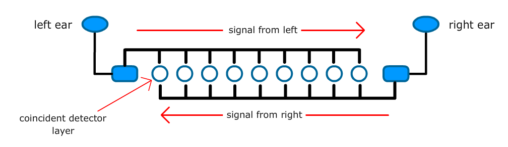
- Click Start.
Imagine that a sound pulse is generated at the moment you click the button, and that it originates from straight ahead. The sound propagates to the ears, and arrives at both ears simultaneously, 4 ms later. This is simulated by the stimuli applied to N1 and N2. These both have a delay of 4 ms, and have been set to each generate a single spike in their respective auditory neurons. These are visible in the top 2 traces in the Results view (at reduced gain).
The spikes conduct to the CD layer, but the spike from the left ear arrives in N3 before the spike from the right ear, because of the different delay lines. The EPSPs summate, but not completely because they are not coincident. The same is true for N4, although the summation is greater.
However, at N5 the spikes arrive simultaneously, and the EPSPs are coincident and they summate completely, and the neuron spikes. A spike in N5 of the CD layer is interpreted by the higher brain processing mechanisms as indicating that the sound came from straight ahead (or behind – the mechanism does not solve that ambiguity).
- Click the down arrow on the spin button for the delay to stimulus 2 to reduce it to 3 ms (i.e. reduce it by 1 ms).
The sound now arrives earlier in the right ear (at 3 ms) than the left (still at 4 ms), indicating that the sound came from the right.
Now N5 is silent but N4 spikes. The brain now knows that the sound came somewhat from the right!
Task: Try various combinations of sound stimulus delay for both stimuli (only change in 1 ms steps for this simulation). See if you can predict which neuron will spike in the CD layer (if any) for your chosen combination of delay.
Take-home message. The Jeffress mechanism relies on two key circuit features. First, an ordered map of delay lines projecting from left and right receptors to the coincidence detection layer. Second, the neurons in that layer do what the name suggests, they act as coincidence detectors. They have brief EPSPs and rapid time constants, and they only spike if there is complete temporal summation of their inputs.
Phase Ambiguity
We will now look at a slightly more sophisticated implementation of the Jeffress mechanism. This is more realistic, although still a long way from the complexity of a real nervous system.
- Load the parameter file Jeffress 1 (v5-2).
The circuit is very similar to the previous one, but there are more neurons in the CD layer and the stimuli are different. The same rules apply regarding synaptic delay.
- Click Start.
The Results view shows the two auditory neurons (N1 and N2). This time the sound stimulus is a continuous pure-tone sine wave with a period of 3 ms, giving a frequency of 333 HzThis is somewhat above middle C on a piano, but below the Stuttgart tuning pitch of A at 440 Hz (showing off!).. The sound arrives at the left ear (N1) 4 ms after you click the Start button, and at the right ear (N2) 5.5 ms after the click, giving an ITD of 1.5 ms. This is half the period of 3 ms, so there is a 180° phase difference in the sound wave at the two ears. This is visible in the stimulus monitor (lower trace). It corresponds to a sound originating from the left side (calculating exactly where would require doing some geometry and knowing the head size and speed of sound, so we won’t bother).
Both N1 and N2 show sinusoidal oscillations in response to the stimulus, but they only spike occasionally They both usually spike on the first sine wave peak, but after that much less frequently. The increased probability of spiking to the first sine wave is due to the low-pass filtering properties of membranes, which enhance the initial transient response to a varying input signal.. This is because the peak of the sine wave is very close to the spike threshold, and, because there is some membrane noise in the neurons, the peak of the sine wave sometimes crosses threshold but usually it does not. (See the tutorial on stochastic resonance for more details on how noise can benefit sensory detection.) However, when the neurons do spike, the spike is always quite tightly synchronized to the peak of the sine wave. This is similar to how real auditory neurons behave. When either neuron spikes, an EPSP occurs in N3, which is the left-most neuron in the coincidence detection layer (the remaining neurons are not shown). However, the EPSP from a spike in N1 (the left ear) will have a shorter latency than the EPSP from a spike in N2 (the right ear), due to the difference in the conduction delay from the two sources.
- Click Start repeatedly a few times, and observe that the occurrence of spikes in N1 and N2 is randomAs stated before, there is usually a spike on the first cycle of the stimulus due to the low-pass filter characteristics of the membrane, which make the first cycle of the sine wave slightly larger than subsequent cycles., but, as stated previously, the spikes always occur at or near the peak of the sine wave.
Task: When you see an EPSP in N3, identify which pre-synaptic neuron (N1 or N2) generated it, based on the latency. Activating a vertical cursor (click the toolbar button ![]() ) might help clarify the timing.
) might help clarify the timing.
An important feature of the signal processing is now apparent – phase ambiguity. There is a clear difference in the time of arrival at the start of the sine wave (the transient disparity, reflecting the different delays set for the stimuli) so this would be a good measure of ITD. However, this generates a single spike at best in each neuron. After that, the disparity in the continuing signal (the ongoing disparity) is ambiguous. Because the sensory neurons do not spike on every peak of the sine wave, and because it is random which peaks they do spike on, spikes in the two neurons separated by 1 sine-wave period might reflect a genuine ITD of 3 ms, or it might reflect an ITD of 0 ms where spikes just happened to occur on successive peaks, or, indeed, the real disparity could be any multiple of the period.
- Load and Start the parameter file Jeffress 2 (v5-2).
This is exactly the same circuit and stimulus, but the Results view is different. We are now looking at just the spikes, which are each represented by a dot, and we can see the activity of all the neurons in the circuit. The top 2 neurons (red and blue) are the auditory receptors, and these spike quite frequently (the dots are close together), while the remainder (green) are neurons in the CD layer, and these spike less frequently.
Let the simulation run for a while, and look at the spikes in the neurons in the CD layer. Hopefully, you will start to see that there are two diffuse “bars” of dots (spikes) centred around N9 and N16. These rows have a higher density of dots than the intervening rows around N4, N12, and N20.
This can be shown more clearly as follows.
- Click Clear.
- Click the Spike frequency graph box at the bottom of the Display mode group in the Results view.
This activates a new dockable window, the Spike Frequency display. It should already be set up with the X axis representing neurons 3 – 21, i.e. the neurons of the coincidence detection layer.
- Move the Spike Frequency dialog so that it does not obscure the Results (you can increase its size too, if you wish and have a big enough screen).
- Click Start.
The Spike Frequency window shows a bar chart of the cumulative spike frequency of each neuron in the CD layer, which updates as the simulation progresses. After a while it should be clear that there are peaks in frequency centred around neurons N9 and N16, and troughs at N4, N12 and N19.
- Click Clear.
- Change the stimulus 2 delay to 4 ms (the same as stimulus 1). This gives an ITD of 0 ms.
- Click Start.
The sound waves are now arriving simultaneously at the two ears, so this corresponds to a sound origin on the midline. The peaks in the graph now occur where previously there were troughs, and vice versa. The network can discriminate between the two sound origins!
Two things might immediately strike you about this simulation. First, there is a lot of random noise in the timing of spike occurrences, so it takes quite some time to establish the true pattern. This actually reflects the experimental findings when recording from individual neurons in the CD layer in owls, where the Jeffress-like output is only established over multiple trials. However, since the owl can determine sound location very rapidly, it is likely that in the intact animal there are many similar circuits operating in parallel, and that the animal can rapidly establish the true pattern by averaging the outputs of these circuits.
The second noteworthy feature is that there are multiple peaks in the graph. The sound has a single location, but the output seems to be ambiguous.
- Click Clear.
- Change the stimulus 2 delay to 7 ms. This gives an ITD of 3 ms, which is the same as the cycle period.
- Click Start.
The sound is now coming from the extreme left, but the output is the same as that generated by sound from the midline. The output is definitely ambiguous!
For comparison the outputs are shown below, with different colours for the different sound origins. These graphs are very similar in shape to those published as Figure 12 by Carr and Konishi (1990).
a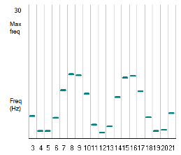 b
b 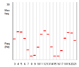 c
c 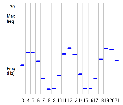
What is going on?
Remember that we are using a pure-tone sine wave as a stimulus, and that individual sensory neurons spike randomly on the peaks of the wave. With the midline origin and extreme left origin, the simulation is set up so that the difference in time of arrival is exactly 1 period of the sine wave, so apart from the very first cycle, the sine waves are identical at the two ears! However, even when the waves have a phase offset, it is not possible to distinguish between sound locations whose time of arrival differ by a whole cycle period. Hence the multiple peaks on the graphs.
This phase ambiguity can be demonstrated in intact, live animals, but only if they are given a pure-tone stimulus. In an experiment with such a stimulus, the bird will be confused and choose randomly between different locations at fixed angular intervals. So it is not a problem with the model, it is a problem with the animal! However, pure tones are very rare in nature, and as soon as the sound stimulus contains mixed frequency (like the white noise of a rustling sound) the animal can determine sound origin very accurately.
How do mixed frequencies resolve phase ambiguity?
There is good evidence that there are multiple Jeffress circuits, with each one tuned to a particular sound frequency. So with a pure tone, only one gets activated. If there is a mix of 2 tones, 2 circuits get activated. Both these circuits show phase ambiguity, but the peaks have different separations, corresponding to the different periods of the stimuli.
- Load the parameter file Jeffress 3.
In this version of the model, a second set of auditory neurons (N22 and N23) and a new CD layer (N24 – N42) have been added. These are identical to the original set, but the auditory stimulus frequency has changed. The new stimuli (3 and 4) each produce sine waves with a period of 4.5 ms, giving a frequency of 222 Hz rather than the 333 Hz of the first setThe amplitude of the lower-frequency current is also slightly lower, so that it produces the same sized voltage deflection as the higher frequency stimulus in the sensory neurons. Remember that the neural membrane acts as a low-pass filter due to its RC properties, and without the change the higher frequency would produce a smaller response.. The ITD is the same as the first set because the speed of sound is independent of its frequency.
A third layer called the integration layer has been added. This receives mapped excitatory input from equivalent neurons in both CD layers; i.e. the leftmost 333 Hz CD neuron and the leftmost 222 Hz CD neuron both make input to the leftmost integration layer neuron, and so on.
In this implementation the integration layer neurons are not coincidence detectors. In fact, the EPSPs are a different type (type b) compared to those impinging on the coincidence detectors, and they are sufficiently large that they initiate a spike in response to input from either CD neuron. The integration layer thus acts as a logical-OR integrator (this is not based on experimental evidence; it is in fact just a hypothesis about how the system might work).
- Activate the Spike frequency graph window by clicking its check box in the Results view.
Note that the graph is monitoring neurons in the 333 Hz CD layer (N3-N21).
- Click Start and run the simulation long enough for the frequency graph to stabilize.
We already seen this result – there are two peaks of similar height in the graph, which thus demonstrates phase ambiguity as before.
- Change the graph colour to blue by clicking the Bar colour button.
- Change the graph Neuron monitor list to 24 - 42 so that it shows activity in the 222 Hz CD layer neurons.
- Click Clear and then Start.
Note that the right-hand peak is in the same location in both CD layers, but the left-hand peak is shifted to the left in the 222 Hz layer compared to the 333 Hz layer.
- Change the graph colour again, perhaps to green.
- Change the graph Neuron monitor list to 43 - 61 so that it shows activity in the integration layer neurons.
- Click Clear and then Start.
The output of the3 layers is shown below. Note that in the integration layer graph (on the right below) the vertical scale has been changed.
a 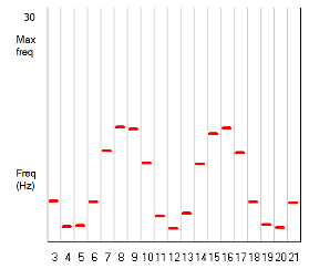 b
b 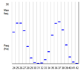 c
c 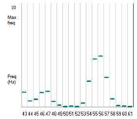
In the two CD layers, only the “correct” peak (the right-hand one) is in the same location, so when activity is summed in the integration layer, this peak is enhanced. The other peaks flatten out, as the peak in one CD layer coincides with a trough in the other CD layer. And thus the summed output of the integration layer has a single dominant peak in the correct location, and the ambiguity can be resolvedWith just two frequencies being integrated there is still a small but definite peak in the 'incorrect' location. However, hopefully you can see that if there were multiple frequencies the multiple incorrect peaks at different locations would flatten out to a stable baseline, with just the 'correct' location showing a significant peak..
Learning Networks
In its simplest form, the Hebb rule for synapses says that if a neuron fires a spike shortly after a pre-synaptic neuron excites it though a Hebbian synapse, then that synapse is strengthened. This simple concept forms the basis of many theories regarding learning mechanisms, although the mechanism that actually implements Hebb learning is still much debated.
Classical Conditioning: Pavlov’s Dog
At a Hebbian synapse it does not have to be that synapse itself that triggers the post-synaptic spike to enhance the connectivity, a completely separate excitatory input can have the same effect. All that has to happen is that the cell post-synaptic to the Hebbian synapse spikes shortly after the Hebbian synapse is activated.
Hebbian synapses can thus provide a cellular mechanism analogous to classical (Pavlovian) conditioning.
In the Setup view we see three neurons that we will pretend exist in the brain of one of Pavlov’s dogs. [This is very much a concept diagram – it certainly does not reflect reality!] In the Results view we see recordings from these neurons.
N1 (top trace) is an olfactory meat detector. It spikes when a meat stimulus (stimulus 1 in the Setup view) is delivered: this is the unconditioned stimulus (US). N1 makes a strong excitatory synaptic connection to N2.
N2 (middle trace) is a command neuron in the saliva-producing motor path. It spikes when it receives an EPSP from N1, and when it spikes it makes the dog drool (remember, we’re just pretending that such a neuron exists).
N3 (bottom) is an auditory neuron that responds to ringing a bell, which is the conditionedI HATE this terminology. It is the response that is conditioned, the bell stimulus does the conditioning. So it would make much more sense to call the bell a conditioning stimulus. However, my objections are not going to change more than 100 years of usage! stimulus (CS) which does not normally elicit saliva. A bell is rung 3 times at fixed intervals, producing spikes in N3. N3 makes a weak Hebbian excitatory input to N2, which is visible as small EPSPs following each N3 spike.
Note that the smell of meat (N1 spike) elicits saliva (N2 spike), while subsequent bell-ringing (N3 spikes) does not. Thus when the US precedes the CS, the CS does not show any response augmentation. So far so good.
- Increase the delay to the US by changing the Stimulus 1 delay from 52 to 152 ms.
- No need to click Start because Options: Run on change has been selected.
The first bell-ring now precedes the smell of meat, and subsequent bell-rings produce an enhanced response in N2, i.e. the EPSPs are bigger, causing a greater chance of drooling. However, they are still sub-threshold. The association between bell-ringing and the smell of meat is not strong.
- Reduce the delay by 10 ms steps, by repeatedly clicking the down-arrow of the delay spin button.
As you reduce the delay, you bring the US closer to the CS (the bell sound follows the meat stimulus at a shorter interval). As the interval declines, the bell-induced EPSP gets bigger.
When the delay between the US and the CS is very short, the augmentation increases to the point where the CS elicits a spike. The dog now drools in response to ringing the bell!!
Classical conditioning is an example of the general phenomenon called “associative learning”, in which the nervous system learns an association between two independent events.
Take-home message: In classical conditioning timing matters. In most cases, the shorter the interval between the unconditioned and conditioned stimulus, the more effective the learning process.
(Classical conditioning is an immensely complicated subject that psychologists have devoted much effort to studying. This simulation only gives a very simplified view of one aspect of it.)
Associative Learning: Pattern Completion
Pattern completion is something that we are all familiar with. If we catch a partial glimpse of a familiar object, we have no difficulty in recognizing it and reconstructing the entire object from memory. On the other hand, if we only get a partial glimpse of something that we have never seen before, then of course we are completely unable to recognize it (unless it looks sufficiently like a bit of an object that we have seen before, in which case we might make a mistake and think the new object is the old object - and that is a fascinating topic in its own right).
There is a huge experimental and theoretical literature on associative learning and pattern completion, and many detailed and very clever mathematical approaches have been taken. However, many such approaches have some sort of Hebb rule at their heart.
- Load the parameter file Pattern Completion.
This looks like a bit of a spider’s web because there are so many connections, but it is actually a quite simple repeating pattern.
There are 3 layers, each with 10 neurons in it. The top layer is a feature detecting layer. Each neuron in this layer responds to a different general feature in an object. The system starts off not knowing anything, but if enough features are detected simultaneously, then together they are identified as an object, and this will generate an identical output pattern on the bottom layer, the object recognition layer. However, if there are insufficient features to constitute an object, then there is no output. After an object has been recognized, then presentation of just one feature in the object causes the recognition layer to make the same output that it does when presented with the entire object. The network has learned the features of the object, and it can now be recognized from just one of those features – this is pattern completion. Presentation of a single feature not in the original object still produces no output.
The process depends upon Hebbian synapses made by neurons in the middle layer of the network, which we could call the learning layer. I will discuss how it works in a moment, but first let’s see it in action.
- Click Start.
The dots in the Results view represent spikes in the feature detector layer (N1 – N10, top half of display) and the object recognition layer (N21 – N30, bottom half of display). (The learning layer is not shown at this stage.)
A series of stimuli are presented to the feature detectors in 4 sequential stages.
First a single feature is presented to N3 (stimulus 1, latency 10 ms). This generates a spike in N3, but a single feature does not constitute an object, and there is no output from the recognition layer.
Next, 3 features are presented simultaneously to N3, N5 and N7 (stimuli 2, 3, and 4, each with latency 50 ms). Three features occurring simultaneously are enough to constitute an object, and neurons N23, N25 and N27 spike, thus representing that object in the recognition layer.
The network has now learned to recognize the object. In this case learning occurs after just one presentation of the feature set because the synaptic and threshold properties of the network were set up that way. It would be more realistic to require several presentations, but that would just complicate things for this demonstration.
Next a single feature is presented to N3 (stimulus 5, latency 90 ms). This is part of the feature set of the object that the network has learned, and the network reconstitutes the entire object in the recognition layer, and neurons N23, N25 and N27 spike, just like they did to the whole object.
Finally, a new feature is presented to N1 (stimulus 6, latency 130 ms). This is not a feature of the learned object, and it is not a new object itself (a single feature is not an object) and there is no output from the recognition layer.
Hebbian mechanism
A circuit fragment is shown below. The whole circuit is just repetitions of this fragment.
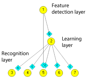
Each neuron in the feature detection layer makes a rather weak excitatory synapse (type a) straight through to its partner in the object recognition layer (vertical connection between N1 and N5 in the diagram). This is not strong enough to make the recognition neuron fire on its own.
Each feature neuron also makes a strong excitatory synapse (type b) to its partner in the learning layer. This is strong enough that whenever the feature neuron spikes, so does the learning neuronIn terms of computational logic this makes the learning layer redundant since it simply duplicates spikes in the object recognition layer. However, its neurons make different types of output to those of the feature layer, and so it is easier to understand the network if it is kept as a separate layer. (N2 always spikes when N1 spikes).
Each learning neuron makes an initially weak Hebbian synapse (type c) to all the neurons in the recognition layer. This is not strong enough, even in combination with the direct activation from a single activated feature neuron, to cause the recognition neuron to spike.
However, if 3 features are presented, each of the 3 recognition neuron partners to the activated feature neurons gets excitatory input from a total of 4 sources; its own feature neuron, the learning neuron partner to its own feature neuron, and the learning neuron partner to the other two feature neurons that have been activated. Each of these is weak, but together the 4 inputs take the recognition neuron above threshold, and it spikes. This enhances the 3 Hebbian inputs deriving from the 3 learning neuron partners to the 3 activated feature detectors. The enhancement is such that now activation of a single learning neuron by a single feature neuron within the object will activate all three of the recognition neurons to which it makes enhanced connections. The recognition neurons can thus reconstitute the original object from just a single feature.
Limitations
This model of course has numerous limitations, one of the most obvious being that it rapidly saturates. If another object is presented that shares features with the first, then that will be learned too and subsequent output when presented with a feature from either object will be a mixed representation of both objects. To solve that one could introduce some sort of “competition” between outputs, perhaps by lateral inhibition, so that the recognition layer would be attracted to one or the other object patterns. However, that is far beyond the scope of this tutorial - there are many whole books entirely devoted to exploring possible neural mechanisms for associative memory and pattern completion. But hopefully this simulation provides food for thought, and at least reinforces the importance of the Hebbian concept in learning theories.
Facilities for Memory Models
The Memory menu provides commands that can be used to investigate learning processes in more complex networks. By default, learning is only retained for the duration of a single experiment, so that when the experiment terminates (by running to completion or by clicking the End button), anything learned in the experiment is lost (by the simulation, hopefully not by the user). The Retain Hebb memory command is a toggle that enables training to persist between experiments. This means that experimental conditions such as stimulus parameters can be changed between experiments, while still retaining the network in its trained state. But note that when this option is selected, the circuit itself cannot be altered and nor can the synaptic properties. Related to this facility is the Reset Hebb memory command, which puts all synapses back into their untrained, starting state. The List Hebb memory command allows you to examine the numerical values of the starting condition, current level of training, and potential maximum trained state of all Hebbian connexions. The Randomize Hebbian command sets all Hebbian connexions to some random value between their starting (naïve, untrained) condition and their fully trained state.
A critical period can be defined using the Set critical period command. A critical period is a time window during which learning takes place. Outside of this window, Hebbian synapses act like ordinary synapses. Once the critical period has been defined, it can be activated or de-activated by selecting the Use critical period command toggle. Finally, the Freeze Hebb memory command is a toggle that you can apply during an experiment. If you select this command during an experiment, no further training takes place until you de-select it. The Hebbian synapses are frozen into their current state of learning. This is a useful method of simulating a critical period “on-the-fly” during an experiment.
Wilson-Cowan Firing Rate Models
So far in this tutorial, network models have been made from a relatively small number of neurons, each with its own identity and its own properties, connected to the other neurons through specific synapses. The properties of the network arise from the interactions between these “identified neurons”. However, the nervous system of most animals has at least some regions containing very large numbers of neurons, which can only be distinguished from each other in terms of belonging to a particular category, or sub-population, rather than as individuals. It is unrealistic to try to model each neuron in such a population - instead some models just simulate the activity within sub-populations in terms of their overall spike rate. Such models are called firing rate models, and one of the most famous and influential was devised by Wilson and Cowan (1972). There is a video of Jack Cowan giving a fascinating lecture on the model and its history here. The model has had a lot of influence in simulation studies of higher brain function, and also higher brain malfunction, such as epileptic seizure.
Background Theory
A unit in a Wilson-Cowan model represents a large but spatially-localized population containing an interacting mix of excitatory and inhibitory neurons. The output from such a unit is two time-varying values, E and I, representing the activity levels of these sub-populations at that moment in time. The variables relate to the average spike frequency within the sub-population, but they are normalized to dimensionless numbers such that a value of 0 represents the background activity in the absence of overall excitation or inhibition. A negative value indicates that the activity has dropped below this background level, while a positive value indicates an activity level above background. The maximum possible activity level that the canonical model can produce is +0.5, while the minimum is -0.5, but the actual range of a particular model depends on the model parameters. This is not the most intuitive normalization, but it is what the equations of the original model produce, and since the model is well embedded in the literature, we will stick with it.
The key concepts underlying the model are as follows. The neurons within the unit have thresholds that vary randomly, with a Gaussian distribution, around some average value. The neurons are connected together randomly, with uniform probability, and the connections are dense enough that any neuron can interact either directly or indirectly with any other neuron in the population. All excitatory neurons excite any neuron to which they are connected, and all inhibitory neurons inhibit any neuron to which they are connected.
There are thus four types of interaction: excitatory-to-excitatory (EE), excitatory-to-inhibitory (EI), inhibitory-to-inhibitory (II) and inhibitory-to-excitatory (IE). Each of these has an average connectivity coefficient, or weight, wEE, wEI, wII and wIE, which represents the average number of synapses mediating that type of interaction per neuron. The strength of input to a sub-population thus depends on the activity level of the source sub-population E or I, multiplied by the weight of the interaction that mediates the input. The output of a sub-population depends on the balance of excitatory and inhibitory input that it receives.
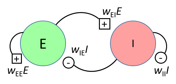
These concepts were formalized by Wilson and Cowan into a pair of coupled differential equations. The justification for this was quite complex, but the final equations \eqref{eq:eqWilCowE} and \eqref{eq:eqWilCowI} are quite simple, and their solution yields the activity levels of the state variables, E and I.
\begin{align} \label{eq:eqWilCowE} \tau_e \frac{dE}{dt} &= -E +(k_e -r_eE) *\Re_e(w_{EE}E -w_{IE}I +X_e) \\[1.5ex] \label{eq:eqWilCowI} \tau_i \frac{dI}{dt} &= -I +(k_i -r_iI) *\Re_i(w_{EI}E -w_{II}I +X_i) \end{align}On the left-hand side, the time constant τ sets the rate at which the activity level decays to the background level if all input is removed. On the right hand side, r is the absolute refractory period. For simplicity, Wilson and Cowan gave this a value of 1 throughout their analysis, and Neurosim does the same. So it can be ignored from now on. The value k is dependent on the maximum activity level, and we will come back to this shortly. The symbol \(\Re\) denotes the response function \eqref{eq:eqWilCowResponse}, which is a function giving the fraction of the sub-population receiving above-threshold input. The argument to \(\Re\), contained within the brackets to the right of the symbol in \eqref{eq:eqWilCowE} and \eqref{eq:eqWilCowI}, is the sum of the within-subpopulation excitatory and inhibitory inputs as described in the previous paragraph, combined with any external input X. The external input takes account of factors such as an experimental stimulus, tonic input from some “higher brain region” (a catch-all term meaning an unspecified but necessary source), or input from a subpopulation in a different Wilson-Cowan unit. The overall external input can be excitatory (X is positive), or inhibitory (X is negative).
The response function used by Wilson and Cowan was a sigmoid function, shifted downwards so that \( \Re(0)=0\), as defined by equation \eqref{eq:eqWilCowResponse} below. They point out that any similar sigmoid function would do, but since this is the form frequently used in the literature, we will stick with it.
\begin{equation} \Re(x) = \frac{1}{1 + e^{-\lambda (x-\theta)}} - \frac{1}{1 + e^{\lambda\theta}} \label{eq:eqWilCowResponse} \end{equation}The first (leftmost) part of the right-hand side of this equation defines a sigmoid curve in the range 0 : 1, whose maximum slope occurs at x = θ, and whose maximum slope value is λ. The second part, which could be called the shift parameter, has a fixed value (it is independent of the input argument) determined entirely by the parameters λ and θ. It is numerically equal to the first part when x = 0, so subtracting it from the first part shifts the output downwards so that \( \Re(0)=0\). This means that when excitatory and inhibitory inputs to a sub-population are exactly balanced (the summed argument to \(\Re\) is indeed 0), the output of \(\Re\) is 0 and the sub-population activity relaxesIf dX/dt = -X, equilibrium is reached when X = 0. to its background level, which by definition is 0.
In a physiological context, the parameter θ relates to the average threshold of the population, and the slope λ relates to the variability around this averageIn formal terms, this makes the response function the integral of the probability density of the threshold distribution. (the shallower the slope of the sigmoid curve, the greater the variability). The shift parameter represents the level of background activity. The higher the background activity, the less “room” there is for excitatory input to increase activity, because neurons have a maximum firing rate. This will reduce the fully-activated value of E or I below the value of 0.5, which is the absolute model maximum. This reduction is reflected by the factor k in the derivative equations \eqref{eq:eqWilCowE} and \eqref{eq:eqWilCowI}. Specifically, k = 1 – the shift factor.
Neurosim Implementation
- Activate the Wilson-Cowan model by selecting it from the Models menu (or select it from the start-up splash screen).
A single Wilson-Cowan unit is visible in the Setup view, containing a greenish circle with an E in it representing the excitatory component (sub-population), and a reddish circle with an I in it representing the inhibitory component. The four possible interactions within the unit are indicated by the squares for excitation, and circles for inhibition, attached to the sides of the two components. Thus the square a is the mutual re-excitation that the excitatory component delivers to itself, while the square b is the excitation that it delivers to the inhibitory component. The circle c is the inhibition that the inhibitory component delivers to the excitatory component, and the circle d is the mutual inhibition that the inhibitory component delivers to itself.
The letters a – d represent the strength of the interaction. The actual value is contained in a lookup table.
- Activate the menu item Connexions: Weights to view the look-up table of interaction weights. This dialog is non-modal, and can be kept open if required while adjusting other parameters. But you don’t need to keep it open just now.
The reason for placing the weights in a look-up table is that it makes it easier to edit properties in complex models, so simply changing the weight in the table can immediately change many interactions without having to edit them each individually. However, it means that there is a limit of 26 (a-z) different interaction weights in the Neurosim implementation of Wilson-Cowan models.
- To satisfy any curiosity you may have, click Start to see what the model produces.
With the default parameters, the unit produces oscillations in both the E and I components, with E slightly leading I. We will discuss this in more detail below.
Stable States
Bi-stable output
- Load and Start the parameter file WilCow Bi-stable.
First, just look at the unit in the Setup view.
- Double-click the unit in the Setup view (either within the greenish E component or the reddish I component) to display the Unit Properties dialog box.
- Note that the Initial level is 0 for both E and I components.
- Note that the Tonic input is 0 for the I component, but -0.6 for the E component. We can ignore the other parameters for now.
- The parameters are those used in Figure 5 of the original Wilson & Cowan paper, in case you want to cross-refer to that.
- Close the Properties dialog.
Now look at the Results view. The upper trace shows the level of activity in the excitatory component (E), and the lower trace shows the level of tonic input to the E component. (We are not monitoring the activity of the inhibitory component in this exercise.)
At the start, E has just background activity (the Initial level in the Properties dialog is 0). However, once the simulation starts, the E component receives immediate inhibitory tonic input of -0.6. This causes a drop in the background level of the E unit until it reaches a stable value a bit below the initial background level.
- Without clearing the screen, click the spin button up-arrow of the Stimulus 1 Amplitude. This adds some additional input to the E component. Combined with the tonic input this will give the overal input to E a value of -0.5 , i.e., slightly less inhibitory.
Note that the E level drops to a very slightly less negative value. It receives less inhibition, so hopefully that makes sense.
- Repeatedly click the up-arrow of the Stimulus 1 for until you reach a level of 1.2, observing the Results view at each change.
Note that for several clicks there is very little change in the output, but when you reach a stimulus level of 0.9 (remember, this is superimposed on Tonic input of -0.6, so the absolute amplitude is +0.3), the E level starts to increase significantly, and with the next click it jumps up to a substantially higher level, quite close to 0.5, which is actually the maximum level that any Wilson Cowan model can produce. Further increase in excitation makes the jump occur earlier, but produces only a small additional increase in the E level.
Important: don't forget what the model represents - the value of E is the overall relative activity level in a large population of neurons, not the response of a single neuron.
- Check the Measure box in the Results view.
- Drag the red measurement cursor to the right in the Results, into the region where the activity is stable.
- Click Measure in the dialog.
- Click Plot to open the XY Scatter dialog.
- Select WC E1 stim from the X axis drop-down list.
- Select WC E1 from the Y axis drop-down list.
Both the raw results and the XY plot show that the model essentially has 2 stable states – a low level that is maintained with excitation less than 0.4, and a high level that occurs with greater excitation. There is thus a threshold very similar to that of a spike in a single neuron, and conceptually, the underlying cause is rather similar. In a single neuron the threshold is due to positive feedback from voltage-dependent sodium channels, in the Wilson-Cowan model it is due to positive feedback from mutual re-excitation within the excitatory sub-population. When this reaches a certain level, it drives the population “hard over” towards its maximum level. The detailed characteristics of this depend on the other interactions, but the positive feedback of mutual re-excitation lies at the core.
Take-home message: With these parameter choices, the Wilson-Cowan model displays bi-stability. The excitatory component output takes one of two levels, dependent on the amount of tonic input it receives.
- Close the XY Scatter dialog.
Hysteresis
What happens if we try to reverse the process?
- Load and Start the parameter file WilCow Bi-stable Hysteresis.
This has the same starting conditions as the previous file, but this time there are two stimuli attached to the E sub-population of the unit.
- With Stimulus 1 selected in the list in the Experimental Control panel, repeatedly click the up-arrow of the Amplitude until the E level flips to its high state.
As before, the flip should occur with the stimulus amplitude reaches a value of 1. (Remember, this is superimposed on Tonic input of -0.6, so the absolute amplitude is +0.4.)
- Select Stimulus 2 in the list in the Experimental Control panel.
- Click the down-arrow of the Amplitude, to give it a value of -0.1.
Note that after a delay, a negative stimulus now adds onto the positive value of the stimulus 1, so that the total stimulus is reduced. However, the E level remains in the high state, even though the total stimulus is now less than that which was required to flip it into the high state when it was starting from the low state.
- Continue to click the down-arrow of stimulus 2, until the E level eventually flips into the low state once more.
The E level remains in its high state until the total stimulus has reduced almost back to its initial tonic level. We can do a similar plot to the previous one:
- Check the Measure box in the Results view.
- Drag the red measurement cursor to the far right in the Results, into the region where the negative stimulus has had its effect.
- Click Measure in the dialog.
- The values from the 20 sweeps should be visible in the dialog report section.
- Click Plot to open the XY Scatter dialog.
- Select WC E1 stim from the X axis drop-down list.
- Select WC E1 from the Y axis drop-down list.
You should now see a typical hysteresis graph:
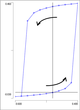
Take-home message: The bi-stable Wilson-Cowan configuration shows hysteresis – a process in which the value of a property lags behind a change in the value of the thing causing it. It is as though the activity level is “sticky”, so that when starting from a low level it takes a big increase in excitation to shift the activity to a higher level, but once there, it takes a big decrease in the excitation to shift it back down again.
- Close the XY Scatter dialog.
Tri-stable output
- Load and Start the parameter file WilCow Tri-stable.
- Double click the unit in the Setup view to open the Unit Properties dialog.
- The parameters are taken from Figure 6 of the original Wilson & Cowan paper.
The model is very similar to the previous bi-stable model, but there are small differences in the weighting and response function parameters, and the level of tonic input.
- As before, repeatedly click the up-arrow of the Stimulus 1, until it reaches a value of 1.0, observing the Results view at each step. Note that the input increases by 0.05 at each step. Do not clear the screen between sweeps.
Note that there are now three stable states in the E activity level – a low value of about 0, a middle value of about 0.2, and a high value of about 0.45.
- Select Stimulus 2 in the list in the Experimental Control panel.
- Repeatedly click the down arrow of Stimulus 2, until it reaches a value of -1.0, observing the Results at each stage.
- Using the same method as described previously, measure the value of E at the right of the Results view for each sweep, and plot the stimulus strength (X axis) against the E activity level.
Task: Identify the points in the graph that are common to the sequence of both the increasing and decreasing stimulus strength, the points that are unique to the sequence of increasing stimulus strength, and the points that are unique to the sequence of decreasing stimulus strength. Thinking this through should help you to understand hysteresis in the system.
Tri-stable mechanism
It is not easy to predict the output of a dynamical system containing 4 interacting feedback loops (which is why we use simulation in the first place), but by separating out the components we can get at least some understanding of how it works.
- Load and Start the parameter file WilCow Tri-stable Details.
- Double click the unit to show its Properties dialog.
- Select the menu Connexions: Weights to show the connection weight look-up table.
- Try to move both dialogs so that they can be seen at the same time as the main Setup and Results views.
First note in the Connection Weights dialog that all the feedback weights used in the circuit (a-d) have been set to 0, so there are no interactions within the population. Next note in the Properties dialog that the Tonic input to E is set to -0.2 as previously, but that in the Setup view an external stimulus has been added to the E sub-population, and this stimulus is selected in the list in the Experimental control panel. Finally, note that there is a flat red line showing in the Results view, which is the level of the inhibitory component (I). With no interactions and no tonic input to I, this is just 0, which is the background level.
- Repeatedly click the up-arrow for the stimulus Amplitude in the control panel until it reaches a value of 1. This will add to the negative tonic input, giving an actual maximum stimulus of +0.8.
The value of E shows a constant-sized step increase in the Results view, which rises and falls in time with the stimulus onset and offset. However, the rise is not instantaneous, but follows an exponential time course. It looks rather like the passive RC response of a single neuron to injected, but remember that it represents the overall activity level of a population of many neurons. The exponential response follows from the core design of the model, which is for a large population of neurons with varying thresholds and in varying states of refractoriness at any moment in time.
- Reset the stimulus amplitude to 0.
- In the Connection Weights dialog, set the value of a to 13 (the original multi-state value).
- This will mediate positive feedback within the E sub-population
- Clear the screen, then press Start to get an initial sweep.
- Again, repeatedly click the up- arrow for the stimulus Amplitude, until there is a big change when the stimulus reaches a value of 0.4.
With this stimulus, the E level shoots up to a maximum (rather like the rising phase of a spike), and it stays there even after the stimulus terminates. This is because the E population now has recurrent excitation (positive feedback) with non-zero weight, so when the level of activity reaches a certain value, it becomes self-reinforcing and rapidly accelerates to its maximum value. Furthermore, it stays there, because it is now self-sustaining and no longer needs a positive stimulus.
- Reset the stimulus amplitude to 0.
- In the Connection Weights dialog, set the value of b to 20 (the original multi-state value).
- This will mediate excitation onto the I sub-population.
- Clear the screen, then press Start to get an initial sweep.
- Again, repeatedly click the up- arrow for the stimulus Amplitude until it takes off.
The E response is exactly the same as before, but now the I response also takes off, because it receives excitatory input from E. However, it does not have any feedback connection to E, so the I activity has no influence on E (or on itself, since there is no recurrent inhibition yet).
- With the stimulus staying at 0.4, click the up arrow for the type c connection in the Weights dialog, until it reaches a value of 3.
- This will mediate negative feedback from the I to the E sub-population.
At this point, there is a sudden drop in the E and I levels. They both oscillate vigorously, but the oscillations are damped and the activity level stabilizes after a short time. Furthermore, the system now returns to its initial state after the termination of the stimulus.
The introduction of negative feedback inhibition through the connection weight c evidently produces a new, mid-level, response that is stable with this level of stimulation. It diminishes the level of E activity, which in turns diminishes the I activity, but a stable state is reached considerably above the resting state, but well below that of maximum activity that results from only positive feedback.
- Finally, click the up arrow for the type d connection in the Weights dialog, until it reaches a value of 2.
With each increase in inhibition within the I sub-population, the oscillations in E and I stabilize more quickly. It was not obvious in advance that this would occur (at least to this author), but it seems that the mutual inhibition within the I sub-population damps the oscillations within it. There is also a rather counter-intuitive increase in the stable I activity level as the mutual inhibition increases. It appears that the initial reduction in I due to increased mutual inhibition within the sub-population releases E from inhibition, which then leads to greater excitation of I, resulting in an overall increase in the I level, despite the increased inhibition!
We are now back to the original configuration which resulted in the tri-stable output. Which is a good point at which to move on.
Oscillations
- Load and Start the parameter file WilCow Oscillator.
- Double-click the unit in the Setup view to open its Properties dialog.
- The parameters for this model are taken from Figure 11 in the original Wilson and Cowan paper.
We have a Wilson-Cowan unit whose E component receives Tonic input of 1. This creates a stable depolarization in the E unit throughout its duration, accompanied by a very small increase in I due to the EI interaction, but nothing very interesting happens.
- Click the up-arrow on the Tonic stimulus to the Excitatory population to increase it to 1.1.
The unit now oscillates. It takes a short while for the positive-feedback excitation in E to build up, but when it “takes off” it increases activation of the I sub-population, and this feeds back onto E to shut it down. The loss of excitation of I reduces its inhibitory effect, allowing E to escape again. And so it goes on.
- Click the horizontal magnify button in the Results toolbar (
 ), and drag over one of the peaks in the green trace to expand the timebase. This lets you see the relative timing of the E and I activity more clearly.
Conceptually, the oscillation mechanism is rather similar to that of some single-neuron endogenous bursters. In the case of a burster the oscillation may result from the interaction between a voltage-dependent calcium current mediating positive feedback and a calcium-dependent potassium current mediating delayed negative feedback. In the Wilson-Cowan oscillator, the E population mediates positive feedback by exciting itself, and the I population mediates negative feedback because it inhibits E, but with a delay because the I population is only activated by the E population.
The EE, EI and IE connections are all necessary for the oscillations, but the II recurrent inhibition is not essential.
- In the Properties dialog, change the Inhibition weight type of the Inhibitory population from d to z.
This sets the II weight to zero. The system still oscillates, but at a lower frequency. However, the frequency could be increased by increasing the Tonic input level.
Take-home message: With appropriate choices of parameter values, the Wilson-Cowan model can produce rhythmic oscillations in activity level.
Phase Plane Analysis
As described for the reduced Moris-Lecar model earlier, there is a well-developed mathematical framework known as phase-plane analysis for investigating the properties of dynamical systems involving a pair of coupled differential equations. This can tell whether the system is stable, multi-stable, oscillatory, chaotic, explosively unstable etc. Since the Wilson-Cowan model is just such a system of paired equations it is amenable to this analysis, which is one reason why the model is so popular (the other being that it yields valuable insights into real-world problems in neuroscience).
Mathematical analysis in the phase plane is beyond the remit of this tutorial (and the capability of its author), but in its simplest form it just involves plotting the two state variables of the equations (E and I) against each other to produce what is called a phase portrait. This gives an alternative view of the shape of the system response, which can emphasise features that are not immediately obvious in a normal time-series plot.
- Reload the WilCow Oscillator file to return to starting conditions, and re-open the Properties dialog.
- In the Results view, check the box Phase plane graph (located below the buttons at the top-left of the view).
The Phase Plane graph appears in a new window. You may need to move it so that it does not obscure any controls or results.
- Click Start.
A rather small vertical line appears at the bottom-left of the Phase Plane graph. This reflects the fact that E increases during the stimulus, causing a shift along the Y axis, whereas I remains almost constant at 0, hence no shift on the X axis.
- Click the up-arrow on the Excitatory Tonic input to increase it to 1.1.
The phase plane plot is now very different. We can see this more clearly by expanding the plot and (probably) slowing the simulation.
- Check the Autoscale X and Y boxes in the Phase Plane view.
- Set a slow-down value in the main toolbar. The best value depends on the speed of your computer, but you can experiment to find out.
- Click Start.
You can now observe the phase-plane plot evolve as the simulation progresses. It starts at the bottom-left because the Initial level of E and I is set to 0. As the Tonic input takes effect it climbs up gradually as the E value increases, and then swings into a series of identical clockwise loops, which superimpose exactly on each other, during the oscillations.
While the simulation runs the phase-plane plot is in black-and-white, but once it terminates, it becomes colour-coded by time (if the Colour time box is checked), with blue being the start, and yellow the end time.
The evolution of the phase plane can be seen more clearly in a 3-D plot.
- Click the 3 D button in the Phase Plane view.
- A new window opens containing a 3-D plot of the phase plane data.
- Click the Front button to see a face-on plot, which is identical to the original 2-D plot.
- Drag the plot with the mouse to examine it from different viewpoints.
- Click the Default button to return to a slightly oblique view.
- Click the Auto Y button to set the graph rotating while you sit back and enjoy the view.
- Click Close to dismiss the 3-D plot.
Phase plane loops like this are called a limit cycle, and they are indicative of oscillatory behaviour. Limit cycles are examples of attractors, because they indicate a state that a dynamical system will end up in, even from a wide variety of starting conditions.
- In the Properties dialog, set the Initial level of E to 0.4, and observe the phase plane plot. [Note that you will not see the full plot until it auto-scales at the end of the run.]
The plot now starts at the top-left of the graph, but is attracted into the same limit cycle.
- Set the Tonic input to E to 1.7.
The plot still displays a limit cycle, but spirals round a few times before it achieves it. This is apparent in the normal Results view as a series of oscillations with decreasing amplitude, which stabilize at a fixed but reduced level.
- Set the Tonic input to E to 2.3.
The Results view shows that the oscillations diminish in amplitude until they disappear completely. In the Phase Plane the plot spirals into a single point. This new attractor is called a stable focus.
- Click the 3 D button in the Phase Plane view again. Note that the plot has a spiral funnel shape, with the funnel diameter eventually decreasing to a simple line.
Multi-Unit Models
A Wilson-Cowan unit represents a large but local population of neurons, such as a small chunk of cerebral cortex, or neurons within a segmental ganglion in an invertebrate. However, it is obvious that such local populations may be able to interact with similar nearby populations. This can be modelled using multiple Wilson-Cowan units, with connections between the E and I sub-populations of the different units, in exactly the same way as the connections are made within a unit.
- Load and Start the parameter file WilCow Paired Oscillators.
There are a pair of Wilson-Cowan units, each of which oscillates due to mechanisms described in the previous section. However, the Tonic input to E is slightly different between the two (1.74 to E1, 1.70 to E2), so they oscillate at different frequencies. At this stage there are no connections between the units, so they operate completely independently.
The top axis shows E and I of unit 1, the middle axis shows E and I of unit 2, and the bottom axis shows E of 1 and 2 superimposed. The difference in frequency is obvious in the bottom trace, where the E activity starts in phase, but then drifts out of phase as time passes.
- In the Results view, check the box Phase plane graph located below the buttons at the top-left of the view
- In the Phase Plane dialog, select WC E1 from the Y axis drop-down list and WC E2 from the X axis drop-down list.
- Check the Autoscale X and Y options.
- Click the 3 D button to see the twisted oval shape of the phase portraitNote that formal phase plane analysis is not possible because there are more than 2 differential equations (and in this case they are not even coupled). However, the display can be informative in its own right. of E1 vs E2.
- Close the 3 D display, but leave the standard Phase Plane view open.
Synchronizing Oscillations
To synchronize the oscillators, we obviously have to couple them together somehow. Just as within an individual unit, there are four patterns of connectivity that can occur between two units: EE, EI, IE and II. We will try each of these in turn.
- Select the Connexions: Weights menu option to open the Connection Weights dialog. Note that the weight of Type e is currently 0. Move the dialog so that it does not obscure the main views, but leave it open while carrying out the following procedures.
- Select the Connexions: Multi add menu option.
- Click and drag from E1 to E2.
- When you release the mouse, the Inter-Unit Connection Properties dialog pops up.
- Set the Weight type to e
- Click OK to dismiss the dialog.
- Repeat, dragging from E2 to E1.
- Press the ESC key to exit the add connections mode.
The Setup view should now look like this

There is no change in the Results view, because the 0 weight of Type e means that the connections are ineffective.
- Click the up-arrow for Type e in the Connections Weight dialog to increase the weight to 1.
The Results view shows that the oscillators are becoming phase-locked towards the end of the simulation, although they have different amplitudes, and there is a phase lag between the two E values. This is also apparent in the Phase Plane view, where there is an indication of the development of a limit cycle as an elliptical circle late in the plot (the yellow end of the colour coding).
- Click the up-arrow for type e again to increase its weight to 2.
There is now tight phase-locking between the oscillators, and the phase lag is either very short or non-existence. The phase portrait in the Phase Plane view is approaching a diagonal line, although the differences in amplitude prevent it becoming completely linear.
- Click the up-arrow for Type e again to increase its weight to 3.
The oscillations in the E value in units 1 and 2 are now almost identical. The phase portrait is now an almost linear diagonal plot.
- To see what completely identical oscillations look like, select WC E1 from the X axis drop-down list 1 (the same as the Y axis). You are now plotting an oscillating value against itself, and the phase portrait is just a diagonal straight line. Return the X axis to E2 before continuing.
It is evident that mutual excitation between adjacent excitatory sub-populations in oscillating Wilson-Cowan units can synchronize the activity of the units, as was hypothesised at the start of this section. But are there other ways of achieving synchronization?
- Reset the Type e connection weight to 1 and note the return to the semi-elliptical phase portrait.
- Drag the yellow blobs indicating the target output of an inter-unit connections from the E sub-unit to the I sub-unit. Do this for both connections so that the Setup looks like this:
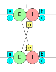
- Click Start.
With E-I coupling between units the Results view shows tighter coupling than was achieved with E-E coupling, and this is confirmed in the phase portrait, which is much closer to a diagonal line. So what about coupling originating from the I sub-units?
- Select the Connexions: Delete all menu command, and click OK in the dialog that asks if you really mean it. We are back with our uncoupled oscillators.
- Select the Connexions: Multi add menu option.
- Click and drag from I1 to E2, and then from I2 to E1.
- Press the ESC key. The Setup should now look like this:
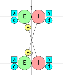
The coupling is even tighter than with the previous configuration. Remember, with EE coupling we needed a connection weight of 3 to achieve tight coupling, but with the IE connection, a weight of 1 achieves similar coupling.
Take-home message: In neural circuits it is often easier to achieve coupling by interactions involving inhibition, rather than through purely excitatory effects. This is probably a general principle of many central pattern generators and rhythmic cortical activity.
Anti-Phase Synchronization
We have seen that three of the four potential coupling patterns (EE, EI and IE) all produce synchronization between units with this parameter set. However, many pattern generators, particularly those involved in locomotion, require anti-phasic coupling between oscillators. Can the remaining untested coupling pattern, II, achieve this?
- Drag the yellow blob indicating the target output of a connection from the E sub-unit to the I sub-unit. Do this for both connections so that the Setup looks like this:
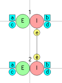
The Results view shows that the oscillations start off in phase, but they rapidly undergo a transition to anti-phasic coupling – when the E1 level is high, the E2 level is low, and vice versa.
The phase portrait is a bit complicated due to the transition, but the red-yellow end of the time spectrum is approaching a repeating skewed figure-of-eight shape, which is a form of limit cycle.
To make this clearer, we could run the simulation for longer. However, another option is to introduce a settling time delay.
- Select the Options: Settling time menu command.
- Set a settling time of 500 ms in the Settling time dialog.
- Close the dialog and click Start.
The simulation now runs for 500 ms in the “background” without displaying anything. This gives the differential equations time to reach the stable limit cycle condition. The figure-of-eight shape of the phase portrait is now very clear. The “waist” of the 8-shape is the cross-over point visible in the Results view, where the two E values are the same. It occurs twice per cycle. The top-left part of the plot is where E1 (Y axis) is high and E2 (X axis) is low, while the bottom right is where E1 is low and E2 is high.
Take-home message: Anti-phasic synchronization can be achieved by coupling the inhibitory sub-populations of a pair of Wilson-Cowan units. Once again, this emphasises the importance of inhibition in neural activity.
Fly larval crawling
The fruit fly (Drosophila melanogaster – the famous animal used as a model system in a multitude of genetic studies) has a soft-bodied larval form known as a grub, and grubs can crawl around using peristaltic waves of contraction generated in the abdomen. There are 8 abdominal segments, and for normal forward locomotion they use waves that start at the back (A8) and propagate forward, and for occasional backwards locomotion they use waves starting at the front (A1) and propagating backwards. The rhythm can be produced by the isolated central nervous system and does not require sensory feedback for its generation, although such feedback can stabilize the rhythm and increase its frequency.
Gjorgjieva et al. (2013) used single Wilson-Cowan units to model the 8 segments of the abdomen, and coupled each unit to its nearest neighbour to achieve intersegmental coordination. They set up reciprocal excitatory coupling between E units in adjacent segments, and inhibitory coupling from each I unit to the E units in adjacent segments.
- Load the parameter file WilCow Fly.
This is an implementation of the Gjorgjieva model (the starting model – they enhanced it with sensory input and bilateral oscillators later in the paper). The intersegmental excitatory connections are the yellow squares showing type e, and the inhibitory connections are the yellow circles showing type f. Note that two stimuli are set up (the white square boxes). Stimulus 1 is applied to A8, and represents brain activation of forward crawling, and stimulus 2 is applied to A1 and represents brain activation of backward crawling.
- Click Start.
Moderately prolonged activation of A8 generates two peristaltic waves that move forward along the abdomen, such as would cause forward crawling in the larva. This is followed by a briefer activation of A1 generating a single backward peristaltic wave. The activity levels in the Setup units are colour-coded, and the peristalsis is visible in the Setup view as a wave of colour propagating along the chain of units. In the Results view the waves are seen as standard changes in E (green) and I (red) activity levels plotted against time.
Take-home message: Appropriate symmetrical inter-segmental coupling can produce peristaltic waves that propagate in either direction, depending on the site of initiation.
The contributions of the intersegmental connections can be seen by editing their weights.
- Select the menu command Connexions: Weights to open the Weights dialog.
- Set type e and f weights to 0 (i.e. effectively remove the intersegmental connections).
Note that A8 produces multiple oscillations. This is because the internal connections of each unit have the original Wilson-Cowan parameters that produce oscillations as described above . The “brain” stimulus provides an episode of tonic excitatory input to A8 enabling 3 cycles of oscillations, while the briefer input to A1 allows only 1 cycle. None of the other units receive any tonic input, so they are silent.
- Set weight type e back to 20, restoring intersegmental excitation.
A wave of excitation propagates along the network, with the same sort of inter-segmental delay as the intact system. The phase progression of the starting model is thus due to the time taken for the excitation to build up to the “take off” threshold in each segment. However, without the intersegmental inhibition, once the E level has taken off, it sticks at the high level.
- Set weight type f to 15, partially restoring intersegmental inhibition.
There are now propagating waves of peristalsis, but they are not of equal duration in each segment, with the initiating segments having longer duration, which diminishes as the wave progresses.
- Set weight type f to 20, restoring the full intersegmental inhibition.
The intersegmental connections are providing some of the same circuit “concepts” as the within-unit connections; mutual excitation and feedback inhibition. Can they actually replace them?
- Set the weights of connection types a and c to 0. This removes the within-unit mutual re-excitation and feedback inhibition.
- Increase the weights of types e and f to 30 to enhance the intersegmental connections carrying out the same function.
The system still produces peristaltic waves with broadly similar properties to those of the starting model. This is interesting, because although the connectivity “concepts” of the two systems have a lot in common, they clearly have rather different connectivity at the anatomical level of actual neurons and synapses. This is another example of the well-established fact that a model may produce an output that looks like that of a real system, but that does not prove that the real system actually works like the model.
On to Kinetics of Single Ion Channels ...