Copyright © W. J. Heitler (2019)

---

Implementation Details

This describes some of the algorithms used in Neurosim.

 

---

Neurons

You can build a neuron with user-specified properties in either the Network or the Advanced HHThe neuron in the HH module itself (not the Advanced HH module) is pre-specified with the properties of the original Hodgkin-Huxley model, and the kinetic properties of the voltage-dependent channels cannot be edited. module. The Advanced HH module has facilities for in-depth investigation and fine-tuning of neuron models which use the HH formalism, while the Network module can incorporate multiple instances of such neurons into circuits, and also includes the option of simple integrate-and-fire neurons.

Hodgkin-Huxley

The Hodgkin-Huxley (HH) formalism assumes that each relevant ion species flows through a separate population of voltage-dependent channels, which individually are either open or shut. The conductance state of each channel depends on a series of independent gates within the channel, each of which oscillates between open and shut states according to 1st-order kinetics, with voltage-dependent transition rate constants. Spikes arise from the properties of these voltage-dependent channels.

Synaptic and stimulus currents are summed with the voltage-dependent currents to determine the overall membrane response.

Integrate-and-Fire

In the integrate-and-fire (IaF) formalism, currents flowing through ion channels and stimulus currents are summed (integrated) and produce changes in membrane potential. If the membrane potential crosses a threshold level a spike 'event' is initiated which triggers appropriate pre- and post-synaptic responses. The spike itself is not modelled (although it generates a cosmetic display), it is just a digital event that lasts for one integration time step.

Note that neurons implementing the IaF mechanism can also contain voltage-dependent channels, but these are not responsible for generating the spike itself.

Neurons implementing the IaF mechanism are generally computationally less demanding than those using the full HH mechanism, and this can speed up the simulation of circuits containing large numbers of neurons. IaF neurons can be used in the Network module, but not the Advanced HH module, which only has a single neuron. The full Hodgkin-Huxley method is a more sophisticated but computationally-expensive approach. It can be used in either the Network or Advanced HH modules.

Neurons built in either model can be saved to disk (file extension nrsm-nrn) and then loaded into either model in a new simulation, although integrate-and-fire properties are ignored in the Advanced HH model. Individual voltage-dependent channels can also be saved and loaded (file extension nrsm-chn).

Passive Properties

The passive neuron is modelled as a RC (resistor-capacitor) circuit, in which the user sets the specific (per unit area) membrane capacitance and leakage conductance. The leakage conductance has a user-specified equilibrium potential, which, in the absence of perturbing factors, will be the resting potential. The user also specifies the neuron diameter, which is used to scale conductance and capacitance to values appropriate for a spherical cell. These parameters are all invariant during a simulation run.
The neuron is perturbed from its resting potential by electrical current. There are 4 possible sources of current:

1. Stimulus current with a variety of waveforms can be applied by the user.
2. Current can pass into a neuron from other neurons to which it is coupled by electrical synapses.

Both these current sources produce size-dependent voltage changes in the receiving neuron, because the response depends on the neuron’s input resistance, which is size-dependent.

3. Current can pass through chemical post-synaptic ligand-gated) channel conductances activated by pre-synaptic neurons.
4. Current can pass through voltage-dependent membrane channels.

The voltage change produced by current through these channel conductances is independent of size, because channel conductance is specified per unit area, and hence the current scales proportionately with size (i.e. ion channel density remains constant as the neuron changes in size).

Noise

The membrane potential can have added voltage noise in the form of a random value drawn from a zero-centred uniform distribution with user-specified range. The noise is added directly to the membrane potential at each integration step, so the quantitative effect is dependent on the step size.

In the Network model neurons can also have added current noise drawn from an Ornstein-Uhlenbeck distribution.  This distribution is a good model for representing background synaptic input with a random mix of excitation and inhibition (Linaro et al., 2011), and is independent of integration step size.

Spiking Properties

In the Advanced HH model the single neuron does not implement the IaF spike mechanism; spikes are entirely generated by HH-type mechanisms.

In Network circuits the user can specify on a neuron-by-neuron basis within a circuit whether to use the IaF model. If IaF is not specified, it is assumed that the neuron is non-spiking, or that spike events are handled by HH-type mechanisms. However, neurons using the IaF spike model can also contain HH-type voltage-dependent channels. These can generate, for instance, low frequency endogenous oscillations such as occur in burster or pacemaker neurons.

With Integrate-and-fire

The neuron has a user-specified spike threshold. If the membrane potential crosses this threshold in a positive direction, a spike signal is generated.

A neuron responds to its own spike signal with a brief (1 integration time step) shift in membrane potential to a user-defined spike peak amplitude. No internal current is modelled during the depolarising phase of the spike, and thus the spike is largely "cosmetic". This is to increase the speed of the simulation, but it can reduce the realism of effects mediated by electrical and non-spiking chemical synapses. The main problem is that the spike is shorter in duration than in a real neuron, which means that less current flows in an electrical synapse. To help overcome this limitation the user can change the strength of a spike which simply changes the effective (internal) spike amplitude, without changing the displayed amplitude.

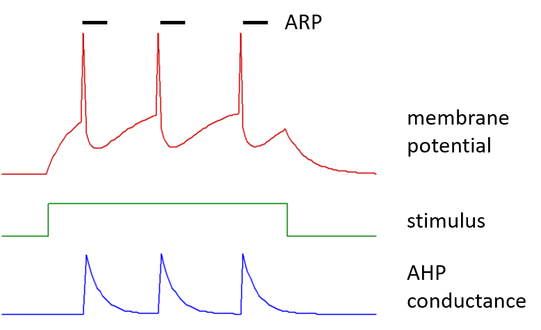
Each spike has an after-hyperpolarization mediated by a step increase in membrane conductance within the neuron, with amplitude defined by the after-hyperpolarizing potential (AHP) conductance. This conductance increase is to an ion with an equilibrium potential defined by the AHP equilibrium potential, which would normally be set to a value appropriate for potassium ions. The AHP conductance then decays exponentially back to a zero value, with a defined AHP time constant.

Following a spike there is a brief absolute refractory period (ARP), during which the threshold is set infinitely high.

A typical IaF neuron is shown below, spiking in response to a stimulus current pulse.

Spike Threshold Accommodation

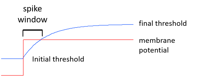
A relative accommodation level can be defined for spike threshold. Accommodation means that spike threshold varies as membrane potential itself varies. An accommodation level of 0 means no accommodation; the threshold is fixed at its defined initial value. An accommodation level of 1 means that when the membrane potential changes, the threshold also changes to eventually exactly parallel the membrane potential and maintain the same relative voltage difference as that between the resting potential and the initial threshold. However, the spike threshold does not change instantly, but rather approaches its new value with an exponential time course, as defined by the accommodation time constant (see figure below). Thus, rapid changes in membrane potential can induce spiking, even if the relative accommodation level is large, so long as the accommodation time constant is long relative to the rate of change of membrane potential.

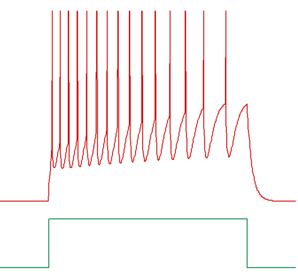
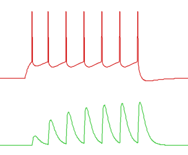
An example of a train of spikes showing threshold accommodation, and hence frequency adaptation, is given below.

 

Synaptic connections

When an IaF neuron generates a spike signal, the signal is sent, with user-specified delay, to all neurons receiving spike-dependent chemical synaptic input from the neuron. This triggers appropriate post-synaptic responses in those neurons.

For neurons receiving non-spiking chemical or electrical synaptic input, the post-synaptic response is a direct function of pre-synaptic membrane potential.

Without Integrate-and-Fire

Spike generation

In a neuron not specified as IaF, spikes may be generated by voltage-dependent channels. Any spike-related properties such as threshold, accommodation, refractory period etc., emerge from the properties of these channels.

Synaptic connections

The non-IaF neuron has a user-specified synaptic trigger threshold for spiking chemical synapses. If the membrane potential crosses this threshold in a positive direction, a spike signal is sent, with user-specified delay, to all neurons receiving spike-dependent chemical synaptic input from this neuron. This triggers appropriate post-synaptic responses in those neurons.

For neurons receiving non-spiking chemical or electrical synaptic input, the post-synaptic response is a direct or indirect function of pre-synaptic membrane potential. Note that the function properties can be set so that only pre-synaptic depolarization which is sufficiently large as to be spike-generated causes a post-synaptic response, thus making the synapse functionally spike-dependent. However, with this implementation the post-synaptic response can depend on properties like pre-synaptic spike duration. This is not possible with standard spiking chemical synapses, which have a duration set by the synaptic properties themselves.

Voltage-Dependent Channels

Each voltage-dependent channel type has a maximum conductance (the conductance when all channels of that type are open) specified per unit area, and the ion to which it is permeant has a specified equilibrium potential. The user does not have to explicitly identify the ion type to which the channel is permeable (but see calcium below), since this is implicit in the equilibrium potential. Thus a non-specific cation channel might have an equilibrium potential of -10 mV as a "compromise" potential between the equilibrium potentials of the permeant ions.

Voltage-dependent channels are usually assumed to be ohmic, and so at any moment in time the following equation applies:

\begin{equation} I_x=g_x(V_m - V_{x\,eq}) \label{eq:eqDrivingForce} \end{equation}

where I_x is the current flowing though the population of channel x, g_x is the overall conductance of that population, V_m is the membrane potential, and V_{eq x} is the equilibrium potential of the ion to which channel x is permeable. The factor (V_m – V_{eq x}) is known as the driving force, and is the equivalent to voltage in Ohm's law.

Non-Ohmic Channels

Channels can be specified to follow the Goldman-Hodgkin-Katz current equation rather than Ohm's Law. In this equation the nominal channel conductance depends upon ionic concentration gradient of the permeant ion. The equation is computationally more expensive than equation \eqref{eq:eqDrivingForce} given above and is rarely used, but it is available if required. More details are given in the Advanced Kinetics section of the tutorial.

All neurons have a leakage channel in which g and V_eq are fixed. However, they may also contain channels in which g varies, depending on the membrane potential, or the intracellular concentration of calcium ions. It is these channels, commonly referred to as voltage-dependent channels, which give neurons their dynamic properties.

In the HH formulation, the variability in g is caused by the presence of one or more gates that can occlude the channel. There can be different types of gate, and multiple instances of each type, within a channel, but all channels of the same type have the same gate population. These gates open and shut in a probabilistic manner, where the open probability depends on the trans-membrane voltage, and in some cases the intracellular concentration of specific ions, particularly calcium. If any gate within an individual channel is shut, then the channel itself is shut (has zero conductance). If all gates within the channel are open, then the channel has its unitary conductance. Because the membrane contains many channels of a particular type, the summed conductance of a channel type is proportional to the maximum conductance (the conductance when all the gates, and hence all the channels, are open), multiplied by the probability of all the gates being open:

\begin{equation} g = g_{max}a^xb^yc^z \label{eq:eqGates} \end{equation}

In this equation a, b and c specify the open probability of 3 different types of gate present in a hypothetical channel, and x, y and z specify the number of gates of each type present in the channel. The gate types, and the number of gates present, vary between the different types of voltage-dependent channels.

In Neurosim there can be up to 9 different types of voltage-dependent channel in each neuron.

Gates

There can be up to 5 different types of gate within each voltage-dependent channel.

The user can specify how many gates of a particular type are present in the channel (the x, y and z parameters \eqref{eq:eqGates}) using the exponent parameter.

For each gate the voltage-dependency of its open probability is described by two equations. As described in the Advanced Kinetics section, the equations can take one of two mathematically-equivalent forms:

1. The equations specify the voltage-dependency of the opening and closing transition rate constants (by convention called alpha and beta respectively). Equations of this form were used in the original Hodgkin-Huxley model.
2. The equations specify the voltage-dependency of the time-infinity open probability, and that of the time constant with which the time-infinity value is approached.

Neurosim provides several different types of built-in equations for specifying these parameters, including those used in the original HH model. There is also an expression parser (muParser by Ingo Berg), allowing the user to write their own equation with the membrane potential as an argument. The parser has many built in functions, allowing a wide variety of equations to be implemented.

Non-Gate Models

Although the concept of gates lies at the core of the physical interpretation of the HH model, some simulations in the literature describe whole-channel conductance directly in terms of its voltage-dependency. This can be replicated in Neurosim by having a channel with just a single gate with a user-defined equation specifying its open probability.

Calcium and sodium channels

The carrier ion of a channel can be specified as calcium, sodium or unspecified.

If the carrier ion is specified as calcium, then intracellular calcium concentration is included as part of the model. This in turn allows the specification of calcium-dependent channels. If the carrier ion is specified as sodium, then intracellular sodium concentration is modelled, which in turn allows modelling the sodium pump current.

Variable Equilibrium Potential

If a channel has calcium or sodium as the specified carrier ion, then its equilibrium potential can be set as variable. This means that it is continuously updated as the simulation progresses, using the Nernst equation and the current value of the intracellular calcium or sodium concentration. The extracellular concentration of these ions is fixed at a user-specified value.

Calcium Dependent Channel

Some ion channels have a conductance that depends on the intracellular calcium concentration, either instead of, or as well as, standard voltage-dependency. Neurosim can include such channels in neuron models, but this requires keeping track of intracellular calcium concentration.

Intracellular Calcium Concentration

Any voltage-dependent or chemical synaptic channel can be specified as having calcium as the current-carrying ion. If this is done, then the current through the channel is a direct measure of the rate of entry of calcium ions, since by definition current is the flow of charge per second.

If we know the current and the cell volume, then in theory we could exactly model the increase in calcium concentration using Faraday’s number which relates charge to the number of ions. However, calcium is not uniformly distributed within a neuron, and in practice a fully explicit model is not easily implemented.

Neurosim models changing calcium concentration as the balance between the rate of inflow and the rate of clearance, using the following equation (Traub, et al., 1991):

\begin{equation} \frac{d[Ca]}{dt}=BI_{Ca}-\frac{[Ca]-[Ca_{min}]}{\tau} \label{eq:eqCaConc} \end{equation}

[Ca] is the intracellular calcium concentration. B is a "fudge factor" that converts the calcium current flowing through ion channels (I_Ca) into a rate of change of concentration. Ionic calcium currents are always inwards in normal physiological conditions, and so the first right-hand side factor BI_Ca describes the increase in calcium concentration due to inflow.

Free calcium is removed at a rate set by its concentration above a minimum value, and the depletion rate constant (\(\tau\)). So the second right-hand side factor describes the decrease in calcium concentration due to sequestration/extrusion. The difference between the two factors is the rate of change of intracellular calcium concentration.

Size Changes

If you want to change the size of a neuron but keep the change in intracellular concentration constant, then the scale factor B should change in proportion to the diameter change - if you double the diameter, double the scale This is because doubling the diameter increases surface area and therefore current by factor of 4, but increases volume by a factor of 8. Doubling the scale halves the effective volume, thus keeping the rate of change of concentration constant.

Making a Channel Calcium Dependent

A channel can be made calcium dependent by adding a gate which has a time-infinity open probability specified in a user-defined equation in which the intracellular calcium concentration is an argument.

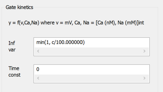
The image above is a fragment from the Voltage-Dependent Channel Properties dialog. A gate called Ca-dependent has been added to the channel, and User-defined inf/tau has been selected for the gate kinetics equation. The Infinity variable text “min(1, c/100)” means that the open probability will be linearly dependent on intracellular calcium concentration (the argument c, which is in nM) divided by 100, but with a maximum value of 1. The Time constant of 0 means that the open-probability will change instantly with a change in calcium concentration. This gate will act in series with any other standard voltage-dependent gates, and will make the open-probability of the channel itself linearly-dependent on the intracellular calcium concentration in the range 0-100 nM, with the probability independent of concentration for values above 100 nM.

The calcium-dependence factor could also be incorporated into a user-defined equation specifying the voltage-dependency of a normal voltage-dependent gate, thus avoiding adding an additional gate to the model. However, the computational overhead of the additional gate is minimal, and there is some advantage to keeping voltage- and calcium-dependency conceptually separate.

Sodium Pump

The sodium-potassium exchange pump (Na/K-ATPase) is an active metabolic pump which uses energy derived from ATP to export sodium and import potassium ions across the cell membrane. It is electrogenic - it exports 3 sodium ions for every 2 potassium ions it imports, and therefore it generates a negative current when active. This current can be included in Neurosim models using the Advanced HH and Network modules. The implementation is largely based on that described by Kueh et al., (2016).

Pump current sodium concentration dependency

A key function of the pump is homeostatic control of the intracellular sodium concentration, and as such, its rate is controlled by this concentration. In Neurosim, the pump current is regarded as a proxy for the pump rate, and the user can specify the current as either a sigmoid or linear function of concentration varying between 0 and a maximum current, or can enter a user-defined equation with sodium concentration (and membrane potential if desired) included as arguments.

Intracellular sodium concentration

The pump current depends on intracellular sodium concentration as described above, and the rate of change of sodium concentration is the difference between its rate of inflow and outflow. Sodium enters the cell through voltage-dependent and/or synaptic channels that have been specified as having sodium as the current-carrying ion. Sodium leaves the cell exclusively through the sodium pump. However, the pump imports 2 units of positive charge (K⁺) for every 3 that it exports (Na⁺), so the rate of export of sodium ions is actually proportional to three times the current generated by the sodium pump. This leads to the following equation:

\begin{equation} \frac{d[Na]}{dt}=B(I_{Na} - 3I_{pump}) \label{eq:eqNaPump} \end{equation}

where I_Na is the sum of currents through sodium-permeant ion channels, I_pump is the sodium pump current and B is a current-to-concentration conversion factor.

If we know the current and the cell volume, then in theory we could exactly model the change in ion concentration using Faraday’s number, which relates charge to the number of ions. Thus if the cell is spherical and there is instant mixing within the entire volume, then each nA of Na current flowing into the cell produces an increase in concentration (mM/s) of this amount:

\begin{equation} \frac{3\times 10^{-6}}{10^{-15}\times 4\pi r^3F} \label{eq:eqFaraday} \end{equation}

However, sodium is probably not uniformly distributed within a neuron, and in practice a fully explicit model is not easily implemented, so Neurosim has a scaling factor that multiplies the explicit factor given in \eqref{eq:eqFaraday}.This generates the factor B in \eqref{eq:eqNaPump}.

Limitations

Neurosim can model dynamic changes in sodium pump current during normal neural activity, and the effects such current has on that activity, but it does not model intracellular potassium concentration, nor does it model extracellular concentrations of either sodium or potassium, which are assumed constant (implying that extracellular volume is infinite). This means that if the pump current is blocked, unrealistic changes in membrane potential can occur, since in reality such a block would eventually lead to loss of intracellular potassium and hence loss of the membrane potential. However, since potassium concentration is not modelled in Neurosim, this does not occur.

 

---

Synapses

Synapses occur in two different modules in Neurosim. In the Network module a wide range of synaptic types can be defined, and used to connect different neurons to each other. In the Advanced HH module there is just a single neuron, and this can receive up to 5 different sub-types of spiking chemical synaptic input. In this module the pre-synaptic sources are not modelled, but the timing of their spikes can be specified.

The following details apply to synapses in the Network module. Where the Advanced HH module is different, this is noted.

There are 3 different classes of synapse available.

1. Spiking chemical class. This is modelled as a brief increase in post-synaptic conductance that occurs at a user-specified delay after a spike in the pre-synaptic neuron.
2. Non-spiking chemical class. This is modelled as a variable change in post-synaptic conductance whose level varies with the pre-synaptic membrane potential or calcium concentration.
3. Electrical class. This is modelled as a non-specific electrical coupling conductance linking two neurons. The current flow from one neuron to the other is dependent on the coupling conductance and the difference between the membrane potentials of the two neurons (i.e. the trans-junctional potential).

Each class can have with multiple sub-types which differ in the quantitative values of their defining parameters.

The Network module can contain an arbitrary number of neurons, and they can be connected by synapses from any of the 3 classes. Each class can have up to 26 different sub-types. Multiple synaptic connections can be made between neurons, allowing mixed synapses to be modelled. An individual synaptic delay can be specified for each connection made with a spiking chemical synapse. In addition, each individual synaptic connection can optionally have a gain modulator which changes its conductance without altering any of its kinetic properties. This can extend the types of connections beyond the 26 sub-types of each class. Individual neurons can also receive random or regular spiking synaptic input from unspecified sources, allowing background synaptic activity to be included in the model.

Spiking Chemical Synapse

A spiking chemical synapse is modelled as a brief increase in post-synaptic conductance that occurs with a specified delay after the pre-synaptic neuron spikes. The post-synaptic conductance has a defined equilibrium (reversal) potential, and this determines whether the synapses is excitatory (equilibrium potential above spike threshold) or inhibitory (equilibrium potential below spike threshold).

Delay

Each connection in the circuit which is mediated by a spiking chemical synapse maintains a delay “pipe”. When a pre-synaptic spike occurs, the delay value is pushed into the pipe. At each iteration of the simulation, all the delay values in the pipe are decremented. When the value at the end of the pipe reaches 0, it is removed from the pipe, so that all other values in the pipe move along one, and the post-synaptic response is triggered.

Shape

The post-synaptic conductance change at a spiking chemical synapse can either have the shape of a single exponential (the fastest option) or a dual exponential. (Advanced HH synapses can also have a square waveform.)

Single exponential

The conductance increase has an instantaneous (i.e. within 1 integration time step) onset to a defined amplitude increase, and then declines exponentially back to zero with a defined decay rate time constant. Note that even though the conductance has an abrupt onset, the resulting voltage change is smoothed due to the membrane capacitance.

 

Dual exponential

The conductance shape is the difference between the exponential curves generated by two time constants; a shorter rise time, and a longer decay time.

Facilitation

Spiking chemical synapses can be specified to be facilitating or anti-facilitating (decrementing). Facilitation is modelled as follows. If a second PSP occurs immediately following a first PSP of the same type from the same pre-synaptic neuron, then the amplitude of the maximum conductance increase of the second PSP is the value of the maximum conductance increase of the first PSP, multiplied by the relative facilitation factor. Thus a relative facilitation value of 1 means that no facilitation occurs, a value greater than 1 means the synaptic response increases (facilitation), while a value less than 1 means the synaptic response decreases (anti-facilitation). As the time interval between two synaptic events of the same type from the same pre-synaptic neuron increases, the degree of facilitation decays back exponentially towards a value of 1 (i.e. no facilitation) with a defined decay time constant. Thus when two pre-synaptic spikes occur, the degree of facilitation depends upon the interval between them, as well as the relative facilitation factor.

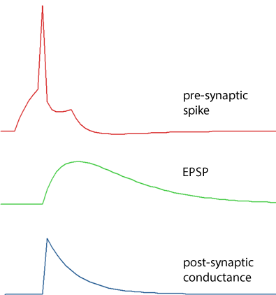
If a series of pre-synaptic spikes occur facilitation is cumulative, so facilitation effects from several pre-synaptic spikes may contribute to each post-synaptic response. In the image below 4 pre-synaptic spikes occur at equal intervals (down arrows). The first spike (red arrow) produces an unfacilitated PSP. The second spike (blue arrow) produces a PSP consisting of its base amplitude (blue), plus facilitation derived from the preceding spike (red). The third spike (green arrow) produces a PSP consisting of its base amplitude (green) plus facilitation derived from the preceding spike (blue), plus residual facilitation derived from the first spike (red). The final spike (black arrow) produces a PSP consisting of its base amplitude, plus facilitation derived from all the preceding spikes, although the component from the first spike (red) is now very small.

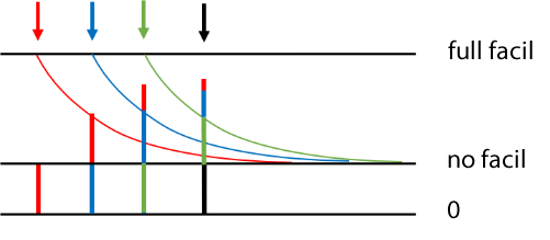
In the Network module this facilitation mechanism produces a fairly realistic qualitative simulation (see image below), but of course this does not imply that the model can be used to fit real data in a quantitative manner.

Voltage-Dependent Synapse

Chemical synapses can be specified as voltage-dependent, if desired. The underlying concept is that the post-synaptic conductance is blocked (e.g. by extracellular Mg⁺⁺ ions in the case of NMDA-receptor channels) when the post-synaptic membrane is relatively hyperpolarised, and unblocked when the post-synaptic membrane is relatively depolarised.

In the Network module the mechanism is modelled as follows. First a nominal non-voltage-dependent conductance is calculated, taking any facilitation into account as described in the preceding sections. This is then scaled by a factor between 0 (fully blocked) and 1 (fully unblocked), with the scaling factor specified as a linear, sigmoid or user-defined function of post-synaptic voltage. In the Advanced HH module the user specifies the minimum (blocked) conductance, and a multiplier that specifies maxium (fully unblocked) conductance. Intermediate conductances can be specified as linear, sigmoid or user-defined functions of post-synaptic membrane potential. The difference between the two modules is simply to maintain compatibility with legacy parameter files.

Hebbian Synapses

Spiking chemical synapses can be specified as having Hebbian properties. A Hebbian synapse is one in which the synaptic strength is dependent upon the degree of conjoint activity of the pre- and post-synaptic neurons. In other words, if the pre- and post-synaptic neurons both spike at relatively high frequency, the synaptic strength is augmented (“trained”). Synapses with these properties are thought to be involved in memory-related processes such as long-term potentiation (LTP) and classical conditioning.

Learning

Learning (augmentation) at Hebbian synapses is modelled as follows. Each Hebbian synaptic type starts from its baseline conductance g_base which is its naive, unaugmented state. Each post-synaptic neuron which receives Hebbian input retains a short-term memory with duration set by the Hebb Time-Window parameter h_wnd in which it records the time of occurrence of any Hebbian inputs which impinge upon it. Whenever such a neuron spikes, it checks its short-term memory to see whether a preceding Hebbian input has occurred within the time window. If such an input has occurred, then the strength of that particular connexion is augmented. The new conductance g_new depends upon 3 factors; the Increment parameter h_incr, how close the current conductance g is to the maximum augmented conductance g_max (specified by the user as a multiple of g_base) and the time t between the Hebbian input and the post-synaptic spike.

\begin{equation} g_{new} = g+h_{incr} \times (g_{max} - g) \times (h_{wnd}-t)/h_{wnd} \label{eq:eqHebb} \end{equation}

The conductance g is then replaced by g_new at the next iteration of the simulation. This means that the shorter the time interval between the Hebbian synaptic input and the post-synaptic spike, the greater the augmentation.

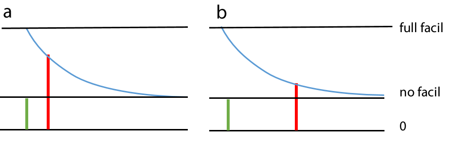
In the image below, a pre-synaptic neuron (top trace, red) spikes twice and mediates excitatory Hebbian input onto a post-synaptic neuron (second trace, green). The first input causes an unaugmented post-synaptic conductance increase (third trace, blue) that reaches the base level g. The Hebbian time window then starts (dashed line). A separate stimulus (bottom trace, green) causes a spike in the post-synaptic neuron, and the second Hebbian input is consequently augmented. If the post-synaptic spike had occurred immediately after the first Hebb input, the augmentation would have reached the level indicated as g_incr (set by the factor h_incr * (g_max – g) in equation \eqref{eq:eqHebb}). However, in the images below there is a delay between the first Hebb input and the post-synaptic spike, so the augmentation is less than the maximum. On the left the post-synaptic spike occurs early in the Hebb window and there is considerable augmentation. On the right, which is a separate experiment, the post-synaptic spike occurs later in the Hebb window, and there is less augmentation.

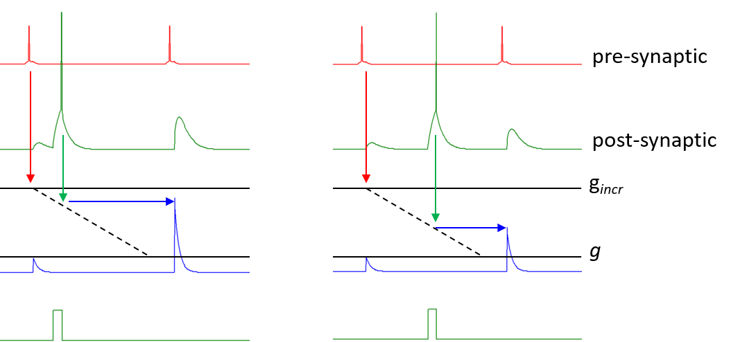
The degree of augmentation is thus linearly dependent on the position of the post-synaptic spike in the Hebb time window.

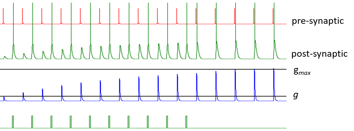
Augmentation is cumulative up to a maximum level g_max, but the increase in augmentation caused by each post-synaptic spike declines the closer the existing conductance g gets to g_max. In the image below there is repeated augmentation caused by repeated post-synaptic stimuli following the Hebb input, but after a while the EPSP augmentation is sufficient to cross threshold in the post-synaptic neuron, and the final few steps of augmentation are self-sustaining, so there is no need for the additional stimulus to induce a post-synaptic spike (see bottom trace)

.

Forgetting

Hebbian synapses can either be set to retain augmentation indefinitely, or to “forget” unless learning is periodically reinforced. Two factors control forgetting; the forgetting time window, and the augmentation factor. The two factors interact, but the former sets a baseline for how quickly synapses forget their training, and the latter determines the degree to which well trained (strongly augmented) synapses forget more slowly than weakly trained synapses. In many ways the augmentation factor resembles synaptic consolidation, but the latter term has mechanistic implications in the field of memory studies, so is avoided here.

Linear forgetting

If the augmentation factor is 1, then the synapse forgets at a fixed rate, irrespective of the degree of training. The augmented conductance simply declines back to baseline linearly during the forgetting time window if it does not receive further reinforcement.

Thus whenever a Hebbian synaptic input occurs the post-synaptic conductance is adjusted as follows. If the time since the most recent Hebbian augmentation (i.e. the time of a PSP in the post-synaptic neuron that got augmented by a following spike) is greater than the forgetting window, then the synaptic conductance is set to its baseline level. If the time is within the forgetting window, then the synaptic conductance is set to a decreased level of augmentation according to the time within the window:

\begin{equation} g_{new} = g - (g-g_{base}) \times t / t_{base forget} \label{eq:eqHebbForget} \end{equation}

where t_{base forget} is the forgetting time window defined by the user, and other symbols are as defined previously. [NOTE: Equation \eqref{eq:eqHebb} is used when a post-synaptic spike occurs to calculate by how much the next input would be augmented if it occurred immediately, while equation \eqref{eq:eqHebbForget} is used when the next pre-synaptic spike actually does occur, to calculate how much of that augmentation has been forgotten.]

Augmentation-reduced forgetting

In general, the more reinforcement a learned process receives, the longer it takes to forget it. In Neurosim this can be implemented at a phenomenological level by specifying that a Hebbian synapse has an augmentation factor greater than 1. For these synapses the baseline forgetting time window is extended by the product of the fractional degree of augmentation and the amount by which the augmentation factor exceeds 1.

\begin{equation} \begin{split} g_{\text{%}} &= (g-g_{base}) / (g_{max} - g_{base}) \\[1.5ex] x_{incr} &= g_{\text{%}}(f_{aug} - 1) \\[1.5ex] t_{forget} &= t_{base forget} + t_{base forget} \times x_{incr} \label{eq:eqHebbConsolidate} \end{split} \end{equation}

where g_% is the current fractional augmentation in synaptic conductance due to Hebbian learning, t_{base forget} is the baseline forgetting time window defined by the user, f_aug is the augmentation factor defined by the user, and x_incr is a local variable holding by how much the base forgetting window gets incremented.

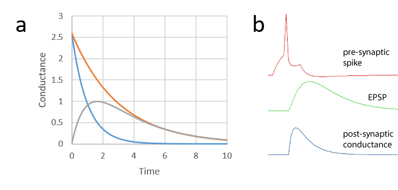
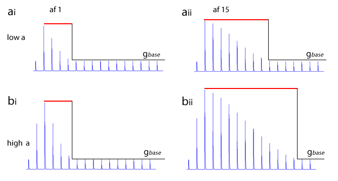
The image below shows the decline in conductance with time of a Hebbian synapse that does not receive reinforcement. The forgetting window is the same for both, but on the left the augmentation factor is 1, on the right it is 20. The initial augmentation is the result of just 1 post-synaptic spike.

Note: The quantitative model for Hebbian synapses used in this simulation is not based on any physiological mechanism. Its only justification is that it produces a behaviour which approximates that which is thought may occur in real systems.

Advanced HH Only

Conductance Decrease Synapse

If conductance-decrease is selected in the Synapse Properties dialog, the resting post-synaptic membrane conductance is increased by the specified synaptic conductance at the start of the simulation, and then this extra conductance is switched off when the synapse is activated. The profile of the conductance change can be specified as for a normal conductance increase synapse, but the synapse cannot be voltage dependent, nor can it facilitate.

Extracellular Calcium Concentration

The user can set whether the synaptic conductance is calcium-dependent. If so, the user sets the ceiling extracellular calcium concentration. At or above this level, the synaptic conductances has its nominal value, but below this level the conductance is reduced in linear proportion to the extracellular calcium concentration.

Quantal Release

To model quantal release at a synapse the user specifies the size of the releasable pool of vesicles, and the average number of vesicles released per activation (the mean quantal content). The actual number of vesicles (quanta) released when the synapse is activated is a random number drawn from a binomial distribution, in which the number of trials is the releasable pool, and the probability of success is the fractional mean quantal content (the mean quantal content divided by the releasable pool).

The post-synaptic conductance change is proportional to the number of quanta, scaled so that the mean quantal content produces the user-specified nominal synaptic conductance.

If the extracellular calcium concentration is reduced below the ceiling specified for maximum release, the probability of release is reduced in linear proportion to the concentration.

Non-Spiking Chemical Synapses

A non-spiking chemical synapse is modelled as a variable increase in post-synaptic conductance whose level depends upon a pre-synaptic control factor, which can be either:

1. membrane potential, or
2. intracellular calcium concentration.

The post-synaptic conductance has a defined equilibrium (reversal) potential, and this determines whether the synapse is excitatory (equilibrium potential above spike threshold) or inhibitory (equilibrium potential below spike threshold).

The relationship between the pre-synaptic control factor and the post-synaptic conductance is called the transfer function.

Neurosim provides two ways of modelling non-spiking chemical synapses:

Direct

The post-synaptic conductance is instantaneously dependent on the pre-synaptic control factor. The user specifies the maximum post-synaptic conductance, and chooses the transfer function from 3 different types. Note that for the user-defined equation, the maximum conductance numerical value could be given explicitly in the user-defined equation, thus by-passing the data edit box value. However, this requires using a conductance value based on the actual surface area of the neuron, whereas the value in the edit box is for a unit area (1 cm²) of membrane, which is consistent with the other types of specifications.

If the pre-synaptic control factor is membrane potential then the post-synaptic conductance co-varies instantly with the pre-synaptic membrane potential. This is the simplest implementation. If the control factor is intracellular calcium, then the post-synaptic conductance kinetics depend on the dynamical control of the pre-synaptic calcium concentration, which can introduce a time delay in the response.

Multi-stage

The concept behind the multi-stage algorithm is that the post-synaptic conductance is dependent on the concentration of transmitter in the synaptic cleft. The pre-synaptic control factor determines the rate of transmitter release with a user-specified transfer function, and thus the rate of increase of concentration. The transmitter is cleared from the cleft at a concentration-dependent rate, with a user-specified time constant which determines the rate of decrease in concentration. The overall change in concentration is the difference in these two rates. \begin{equation} \frac{dConc}{dt} = ReleaseRate - \frac{Conc}{\tau} \label{eq:eqNonSpiking2Stage} \end{equation} The moment-by-moment concentration is determined by numerical integration as the simulation progresses. If the pre-synaptic voltage is stable (\(dConc / dt = 0\)), the concentration reaches a steady state where \(Conc = \tau \times ReleaseRate\).

The post-synaptic conductance is an instantaneous upper-half sigmoid function of transmitter concentration, where the user specifies the maximum conductance and the slope.

Note that transmitter concentration and release rate units are arbitrary - no attempt is made to model actual transmitter concentration realistically.

Carrier Ions: Calcium and Sodium

The fraction of synaptic current carried by sodium and/or calcium can be specified for any chemical synapse (the total must be <= 1). The specified fraction of current is used during the simulation to alter the intracellular concentration of that ion. This can affect both the equilibrium potential for the ion, and also any other properties that are dependent on that ion (e.g. the sodium pump rate, or calcium-dependent ion channels).

Electrical Synapses

An electrical synapse is modelled as a non-specific electrical coupling conductance linking two neurons. The coupling conductance is specified as an absolute value; it is not for a unit area of membrane. This allows coupling between neurons of different sizes.

Current flows from one neuron to the other whenever there is a difference between the membrane potentials of the two neurons (i.e. the junctional potential is non-zero).

\begin{equation} I_{elec} = g_{elec}(V_{m1}-V_{m2}) \label{eq:eqElecSynCurrent} \end{equation}

This current acts in the same way as an external stimulating current, adding excitation to the neuron with the more negative membrane potential, and removing it from the other.

There are two types of electrical synapse:

1. Non-rectifying electrical synapses have a constant junctional conductance irrespective of the membrane potential of either neuron.
2. Rectifying electrical synapses have a junctional conductance which varies with the junctional potential.

Rectifying Electrical Synapses

Rectifying synapses are polarised, and by definition the pre-synaptic neuron is the neuron which acts as a source for positive current (i.e. depolarising potentials pass more easily from the pre-synaptic neuron to the post-synaptic neuron than in the reverse direction). The junctional potential is defined as the pre-synaptic membrane potential minus the post-synaptic membrane potential, and thus the junctional potential is always positive when the rectifying synapse is in the high-conductance state.

Each rectifying electrical synapse has a normal conductance, which is its conductance in the maximum "on" state. This conductance is modulated by the junctional potential according to one of 3 possible transfer functions.

 

---

Equations and Integration

I would like to acknowledge the debt I owe to the book Neural and Brain Modelling by Ronald Macgregor (1987), which introduced me to neural modelling, and in particular the exponential Euler method of numerical integration which is used solve many of the equations in Neurosim.

Exponential Euler Integration

Kirchhoff’s law states that at any point in a circuit the current entering that point is equal to the current leaving it, so the sum of currents is 0. This means that the capacitive current minus all the other currents added together must be 0. This is expressed in the following equation.

\begin{equation} C_m\frac{dV_m}{dt} - (\sum g_x(V_{x \, eq} - V_m) + I_{non\,ionic}) = 0 \label{eq:eqBasicHHForm} \end{equation}

where C_m is the membrane capacitance, V_m is the membrane potential, g_x is the conductance of ion channel x, V_{x eq} is the equilibrium potential of ions flowing through channel x, I_{non ionic} is current entering or leaving the neuron that has not passed through normal ion-specific trans-membrane channels. This latter includes stimulus current applied by the user, membrane noise current, current from electrical synapses, and current from electrogenic pumps such as the sodium-potassium exchange pumpls. It also includes any ionic non-ohmic current generated by the Goldman-Hodgkin-Katz current equation. This equation lies at the heart of all HH-type simulations that have been published, not just Neurosim.

This can be algebraically rearranged thus:

\begin{equation} \frac{dV_m}{dt} = \frac{\sum g_x V_{x \, eq} + I_{non\,ionic}}{C_m} - V_m \frac{\sum g_x}{C_m} \label{eq:eqExpEuler} \end{equation}

[It is worth noting that the driving force expression, which is explicitly present in \eqref{eq:eqBasicHHForm} has been split up in equation \eqref{eq:eqExpEuler} and is no longer obvious (although of course it is still there mathematically).]

Equation \eqref{eq:eqExpEuler} is a linear equation of the form:

\begin{equation} \frac{dV}{dt} = A - VB \label{eq:eqExpEuler2} \end{equation}

where

\begin{equation} A = \frac{\sum g_x V_{x \, eq} + I_{non\,ionic}}{C_m} \label{eq:eqExpEulerA} \end{equation}

and

\begin{equation} B = \frac{\sum g_x}{C_m} \label{eq:eqExpEulerB} \end{equation}

The nice thing about equation \eqref{eq:eqExpEuler} is that the variable in the numerator of the differential, V_m, only appears once in the right-hand side. This means that it can be directly integrated to yield:

\begin{equation} V_{t + \Delta t} = V_t e^{-B \Delta t} + \frac{A}{B} (1 - e^{-B \Delta t}) \label{eq:eqExpEulerStep} \end{equation}

(I must admit that my calculus isn’t good enough to do this from first principles. I’m just taking it on trust from people who can.)

This is the exponential Euler method of numerical integration. It is at the core of the calculation engine because it generates the membrane potential at each moment in time. If we know the membrane potential at the start of an experiment (V_t=0), and we know the value of the variables within A and B at each moment in time, then we can make multiple small steps Δt forward in time and at each step calculate the new membrane potential Vt + Δt, which then becomes Vt for the next step. The main advantage of this method over the basic forward Euler scheme applied directly to equation \eqref{eq:eqBasicHHForm} is that it is stable for much larger step sizes.

HOWEVER, (and it’s a big however), equation \eqref{eq:eqExpEulerStep} is an exact solution only if A and B are constant. In fact, A and B contain factors which may vary with time and voltage (g_x, I_stim and I_elec, etc.), so they too have to be calculated at each integration step.

Integration Components

Intracellular Ion Concentration

The methods for calculating intracellular sodium and calcium concentration changes have been given earlier.

Voltage-Dependent Channels

To calculate g_x for a voltage-dependent channel we multiply the maximum (fully open) conductance of the channel which is specified in the model by the product of the open probabilities (P) of the gates within the channel, as described previously in the Advanced Kinetics section. However, we have to know the values of these open probabilities. For each gate the model will have specified equations either to calculate the instantaneous values of the transition rate constants (α, β), or the time-infinity open probability and time constant (\(P_\infty\), τ).

If α and β are specified, to advance one step Neurosim uses exponential Euler numerical integration of the differential equation given here, which is:

\begin{equation} P_{t+\Delta t} = P_t e^{-\Delta t(\alpha + \beta)} + \frac{\alpha(1-e^{-\Delta t(\alpha+\beta)})}{\alpha+\beta} \label{eq:eqDerivAlphaBetaPStep} \end{equation}

 If (\(P_\infty\) and τ are specified, the equivalent differential equation is given here, with the single-step solution:

\begin{equation} P_{t+\Delta t} = P_t + (P_\infty -P_t) (1 - e^{-\Delta t/\tau}) \label{eq:eqDerivInfTauPStep} \end{equation}

which is just the equation for bounded exponential growth broken up into small steps.

Synaptic Channels

Non-spiking synapses have a conductance that depends on the pre-synaptic control factor, and so they can be included in equation \eqref{eq:eqExpEuler} above. If needed, the synaptic current can be calculated from the driving force.

Spiking Synapses have either a declining single exponential waveform, or a waveform which is the difference between two exponentials. The conductance of each synapse type is incremented by an appropriate amount (taking into account facilitation, Hebbian effects etc.) whenever a pre-synaptic spike occurs, and then decrements at each subsequent integration step:

\begin{equation} g_{syn\, t+\Delta t} = g_{syn\, t} e^{-\Delta t/\tau_{syn}} \label{eq:eqSynCondDecayStep} \end{equation}

where τ_syn is the user-specified synaptic decay rate. Once the conductance is known it can be included in equation \eqref{eq:eqExpEuler} above. If needed, the synaptic current can be calculated from the driving force.

Adaptive Step Size

There is an option to use an adaptive step size during integration in the Advanced HH model. This is a simple algorithm that checks the fractional change in membrane potential and gate open probability at each step, and if it falls below a threshold the step size is increased at the next iteration, or if it exceeds a ceiling the step size is reduced and the step is repeated. The program keeps track of sudden changes such as the onset of a stimulus, and automatically reverts to the minimum step size when they occur. This enables the program to step rapidly through periods where there are only very slow changes in the activity of the single neuron.

This is not used in the Network module because this often includes multiple neurons in a model, and it is unlikely that all the neurons would be showing activity changes at the same rate.

Wilson-Cowan Integration

The differential equations in the Wilson-Cowan model are solved using the standard 4th-order Runge-Kutta method.