Contents
Chart view
Chart view
Trace and view format
Episodic data
Trace gain and position
Data scaling
Viewport
Cursors
Markers and annotations
Scale bars
Multiple views
High-quality figures
Clipboard
Chart view
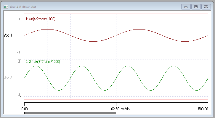
- Load the file sine 4 8. This will be used as the base for the examples described in this section.
Trace and View Format
Data traces are numbered in sequence (1 – n, with a maximum of 128). The number is the ID of the trace. By default, each data trace displays in a particular colour on a separate axis, and optionally has a label associated with it. Each axis also has a label associated with it. These features can be edited.
- Select the Traces: Format menu command to activate the Trace Format dialog.
- If possible, move the dialog so that it does not obscure the main view.
- In the Traces frame, set the trace Label of the top trace (ID 1) to “4 Hz”, and of the second trace (ID2) to “8 Hz”.
- Click the red Colour choice box at the bottom of the dialog, and note how the selected col at the bottom right changes to red.
- Now click the Trace colour box of ID 1 (which was brown) and observe that it turns to red.
- Use the same procedure to set the trace 2 colour to blue.
- Check the Dots box for trace ID 2.
- Normally, each datum point within a trace is joined to adjacent points by a straight line. However, if you want to see the exact sample times and values of a particular trace, you can disable the line, so that each point just draws as a dot.
- In the Axes frame on the right of the dialog, set the axis Label of ID1 to “V”.
- In the same frame, uncheck the Show axis box for axis ID 2 (the lowest of the enabled ID set). This will hide axis 2.
- In the Traces frame, change the Trace axis for ID 2 to show 1. This means that the second trace (i.e. the second data channel) will display on the first axis, superimposed on the first trace.
- If you wanted just to hide the second trace, you would leave its Trace axis set to 2, since this axis will not be displayed.
- Click Apply.
You can now see the effect of the various changes in the main display. Hopefully, they all make sense. You could also just click OK to accept the changes and dismiss the dialog, but with Apply the dialog remains open so you can make further changes if desired, or you could click Reset to undo the changes and start again.
- Click Cancel to close the dialog and undo the changes you made.
- Control-click the gain up toolbar button(
 ) twice to increase the gain of the both axes.
 - Note that the traces now overlap.
- Also be aware that If you had just clicked, rather than control-clicked, the toolbar button, only the selected axis (in this case the upper axis) would have been affected.
- Axes can be selected by clicking on their labels. To select multiple axes, control-click.
- Select the Traces: Format menu command to activate the Trace Format dialog again.
- Check the Clip box for axis 2.
- Click OK.
Now the trace on axis 2 is clipped so that it does not extend beyond the axis scale limits.
- Click the gain up toolbar button( ) to increase the gain of the selected axis 1.
Clip was not selected for axis 1, so this trace now extends beyond its axis limits and overlaps with the trace in axis 2.
You can hide or show the display grid, the trace IDs and labels and the axes using commands on the View menu. You can set the height and width of the display to particular values (in pixels) with the View: Set size command. This may be useful if you want to copy bitmap images of the display with known fixed dimensions.
Line width
By default all traces show with a line width of just one pixel. However, when exporting images for display in other programs this can lead to rather faint traces. You can increase the display line width if desired.
- Select the Traces: Line width: 2 menu command to show the traces with thicker lines.
Dot or Line display
Normally, each datum point within a trace is joined to adjacent points by a straight line. However, if you want to see the exact sample times and values, you can disable the line, so that each point just draws as a dot.
- Set the timebase value to 1 ms/div. The timebase edit box is below the X axis in the middle.
- Select the View: Dots not lines command.
- The dot size can also be set with the View: Dot size menu options.
- Close and re-open the file to return to the starting conditions.
The menu option acts as a global command: all traces display either with lines or dots. If you want to set this option on a trace-by-trace basis, use the Traces: Format menu command to display the Trace format dialog box, and check or uncheck the Dots option for each trace.
Inactive data sections
Some commercial formats, and some data manipulations within DataView, produce traces with sections of inactive data where values are not defined (e.g. the recorder was temporarilly switched off). Such sections are displayed as grey, zero-valued data by default, but can be hidden altogether by toggling the View: Show inactive data sections command.
Data display area
By default, the axes are evenly spread across the vertical height of the view. However, you may want to keep part of the view clear of trace data in order to display events (see below) or annotations.
- Set the View: Data display area to 50% and observe that the trace axes now only occupy the lower part of the screen.
You can still place traces in the upper portion by adjusting their position (see below), but trace data can conveniently be restricted to within axis limits, and hence the lower portion of the view, by using Autoscale on all axes. If you set the Data display area to 0% then all data traces are hidden, although they are of course still present in the file and can be revealed by choosing a non-zero display area.
Time units
The View: Main display time units menu allows you to set the time units of the main display to milliseconds (the default), seconds or decimal minutes (i.e. 1.5 minutes means 1 minute 30 seconds). Different views (see below) of the same file can use different time units, so you can view large sections of a long file using time units of minutes, while simultaneously focussing in on individual spikes using a second view with millisecond time units.
Episodic data
Data can be episodic. In episodic recordings the time-base is not continuous but rather contains episodes of data recorded sequentially in time, but with arbitrary gaps between each episode. Event channel a acts as a marker, with each event indicating the start of a new recording episode. Data can be converted between episodic and non-episodic with the Transform: Episodes menu group. The difference is in whether events in channel a are treated as episode boundary flags, or just normal events.
It may be important to flag episodic recordings correctly because certain analysis and transform procedures need to restart at episode boundaries due to discontinuities in the data waveform.
Trace Gain and Position
You can adjust the gain and/or position of traces by several methods:
- Manually edit the upper and lower settings of the appropriate axis to change either gain or position.
- Click and drag vertically just to the left of the vertical axis line to change the gain. If you drag towards the mid-axis point, you reduce the gain, if you drag away from the mid point, you increase the gain. As you drag, the cursor changes to a magnifier, with + or - at its centre.
- Right-click within the axis region (to the left of the vertical line) and select an option from the context menu.
- Click and drag the trace vertically with the mouse to change its position.
- Click the toolbar buttons to adjust selected axes.
Selecting Axes and Using the Toolbar
Selected axes have their axis labels written in bold type, while non-selected axis labels are written in grey type.
- Select an axis by clicking on the axis label.
- To select multiple axes, hold down the control key as you click.
- You can also select axes using the Traces: Select menu command.
- You can rapidly change the gain and position of traces on selected axes by clicking a toolbar button:
- Gain up ()
- Gain down (
 )
) - Trace up (
 )
) - Trace down (
 )
) - Autoscale (
 )
)
The autoscale button adjusts the display gain so that the largest signal currently displayed on the axis just fills the axis height. This can be useful as a “find trace” facility.
- Gain up (
If you hold down the control key as you click one of these buttons, then the effect is applied to all traces, not just those on selected axes.
- Magnify vertical (
 )
)
If you click this and then drag around a trace, the trace axis adjusts so that the drag box upper and lower levels fill the axis. Note: this can give unexpected (and undesired) results if more than one axis is selected. - Same scale (
 )
)
If several axes are displayed, click this to make all or a selected subset have the same scale settings (position and gain)
This is also available through the Traces: Same scale menu command.
The following rules apply:- If no axes are selected, all axes are set to the same scales as the top axis.
- If one axis is selected, all axes are set to the same scales as the selected axis.
- If several axes are selected, all selected axes are set to the same scales as the top selected axis.
Keyboard shortcuts
The following keyboard shortcuts work on the selected trace:
| Autoscale | control 0 (zero) | |
| Increase gain | + (plus) | |
| Decrease gain | - (minus, hyphen) | |
| Trace up/down | up/down arrow keys |
Data scaling
When DataView reads from a file, it assumes that all voltage values are in units of millivolts, or converts them to this if the file itself contains appropriate scaling information. However, it sometimes happens that numbers from external files are stored in other units without any explicit scaling information. In this case Dataview can scale individual traces as they are read from file.
Imagine that trace 1 of the example file came from a signal generator that produced a sine wave with a peak-to-peak amplitude of 0.1 mV, but that it had been passed through a x10 amplifier before it was recorded. The values in the file would thus be 10 times greater than the real signal.
- Select the Traces: Experimental gain menu command.
- Enter 10 into the trace 1 edit box. This is the gain of our imaginary external amplifier.
- Click OK.
The amplitude of trace 1 has now been reduced by a factor of 10.
Of course, the same scaling procedure can be used even if the original signal represented some factor other than voltage, such as force, or current.
Viewport
The viewport is the section of the total recording that is visible in the chart view. This depends on the display timebase and the display start time.
The grey slider bar under the X axis shows the viewport as a fraction of the total record, where the full width of the axis represents the whole record.
You can adjust the viewport by several methods:
- Manually edit the start time and end times on the horizontal axis.
You can switch between units of millisecond, second or minute with the View: Main display time units menu command. - Manually set the timebase in terms of time per grid division or per viewport (i.e. visible display) by editing the value in the mid position below the X axis at the bottom of the screen.
You can switch between the grid and viewport metric with the View: or Navigation: Timebase metric manu command. - Manipulate the slider bar.
- You can drag the slider bar with a mouse to quickly position the viewport within the file.
- If you drag the left end of the slider bar you specifically adjust the start time
- if you drag the right end of the slider you adjust the end time.
- Click on the main display and drag horizontally to “pan” the display. Do not click directly on a trace or you may move it vertically.
- Click just under the horizontal axis line and drag away from the mid point to expand the display, towards the mid point to compress it.
- Click the Toolbar buttons or select commands from the Navigation menu.
Time vs samples
The first sample point in the viewport displays on the extreme left, while the last sample displays on the extreme right. The viewport time values specify the time between the first and last visible sample, i.e. the summed duration of the gaps between the first and last visible samples. There is therefore one more visible sample than there are gaps.
- Set the end time (right hand X axis scale) to 8 msec.
- Select the View: Dots not lines menu command to toggle the dot/line display to the dots option.
There are 9 dots visible spaced at 1 msec intervals, hence 8 gaps. The start time is 0, and so the end time of 8 msec fits with the data display.
- Reset the end time to 500 msec and select the View: Dots not lines menu command to return to the previous view.
Toolbar navigation commands
Commands associated with navigation are on the Navigation menu (not surprisingly). The most useful commands are also duplicated as toolbar buttons.
- Compress (
 ), Expand (
 )
)
Compress or expand the timebase by a factor of 2. - Show all (
 )
)
This adjusts the viewport to show the entire file. - Magnify horizontal (
 )
)
Click this and drag a box around a section of the display to adjust the start and end times so that the viewport shows just that section. - Go to start (
 )
)
Set the start time to 0. - Go to end (
 )
)
Set the start time to the end time minus the viewport duration. - Page forward (
 ), backward (
 )
)
Increase (forward) or decrease (backward) the start time by the duration of the viewport; i.e. move one page later (forward) or earlier (backward). - Part page forward (
 ), backward (
 )
)
Increase (forward) or decrease (backward) the start time by 20% of the viewport duration.
Keyboard shortcuts
| Compress | / | |
| Increase gain | * | |
| Left/right page | control left/right arrow keys | |
| Left/right page % | left/right arrow keys | |
| Show all | alt 0 | |
| 1 : 1 (one sample per pixel) | alt 1 | |
| Go to start | Home | |
| Go to end | End |
Expand Compress Focus
When you change the timebase you can determine whether the expansion/compression is centered around the left-hand edge or the mid-time of the display using the Navigation: Focus left edge (else mid) toggle command. This command is global; it effects navigation in all open windows.
Cursors
You can position any number of vertical and horizontal cursors on the screen. Cursors are used to make quick measurements of data, and to demarcate sections of data for various analysis procedures. Cursors are not persistent (they are not stored with the data file), and cursors in each view are independent of each other. Cursors do NOT move with the data, so if you pan the data, the cursor stays in the same screen location.
Cursors are controlled through the Cursors menu.
Shortcuts:
Press the keyboard 'v' key to add a vertical cursor to the centre of the view.
Press the keyboard 'h' key to add a horizotal cursor to the centre of the view.
Further details about cursors are given here.
Markers and annotations
Markers
Markers are labelled tags that are associated with a particular time within the file, but not with any particular trace.
- Insert a marker by right-clicking the display and selecting Add user marker from the pop-up context menu (or with the Add ins: Markers: Add menu command).
The cursor changes to an arrow. - Click the time on the screen at which you wish to insert the marker, and optionally enter a text label in the displayed dialog.
You can also set the exact time of the marker in this dialog.
- Click OK, and the marker will be displayed as a purple cross near the top of the view.
- You can also quickly add a marker to the centre of the screen by simply pressing the ‘m’ key.
This marker can then be moved and have a text label added if desired. - You can edit a marker by right-clicking the purple cross mark.
- Markers can be moved by dragging them, unless they are locked (see below).
- You can delete one or all markers using command in the Add ins: Marker menu.
Try adding several markers at different points in the file.
- You can navigate between markers by pressing control m to go to the next marker, or alt m to go to the previous marker.
Annotations
Annotations are like markers in that they display at particular times, but are unlike markers in that each is associated with a particular trace and data values, so they move their vertical position if the trace position moves.
- Annotations are inserted by right-clicking the display, and selecting the Add trace annotation command.
- You can also quickly add an annotation simply by pressing the ‘a’ key.
- You can navigate between annotations by pressing control a to go to the next annotation, or alt a to go to the previous annotation.
- Right-clicking an annotation allows you to edit it.
Try adding an annotation with some text, and then change the position of the associated trace to see the annotation move.
Locking markers and annotations
Both markers and annotations can be independently locked to prevent them being accidentally moved by the mouse.
- To lock markers or annotations check the Add ins: Markers: Lock or Annotations: Lock command.
Some commercial acquisition formats (e.g. CED Spike files) use markers to indicate particular points of interest in the record. These are imported into DataView when the file is read, and such markers are automatically locked. Markers and annotations can be unlocked by unchecking the command above.
Scale Bars
You can add a horizontal (timebase) scale bar, and multiple vertical (amplitude) scale bars to the view. These will show even if the axes are hidden (see the View: Show axes menu command).
The main point of these scale bars is that they are included when the screen display is copied to the clipboard, or when vector format files are exported using the File: Write hi-def graphics commands (see below). This means that if these files are subsequently edited in graphics programs and the traces are scaled by stretching or compressing, then if the scale bars are included in the transform so that there is a continuous record of the scales that can be included in publication-quality figures.
- Click the Show all toolbar button ().
- Select the Add ins: Horizontal scale bar: Add menu command to show the Horizontal Scale Bar dialog.
- Set the Duration to 100 ms.
You can also set the line thickness, and the font (including colour) of the scale bar text label, if desired, but the defaults are suitable. - Click OK.
- Then click the main view at the location that you want to place the left-hand end of the scale bar.
For now, place it in the middle of the view. You can drag the scale bar to a new location if you need to. - Click the expand timebase toolbar button ().
Note that the scale bar expands appropriately. - Click the part page forward toolbar button ().
Note that the data scroll forward, but the scale bar stays in the same screen position. Its location is fixed relative to the window frame, not relative to the data. - Change the physical size of the window showing the data by dragging on a corner of the windows frame.
Note that the scale bar scales appropriately (as do the data themselves, of course).
Vertical scale bars are added by a similar process, but for these you also have to specify which trace the bar applies to. The bar will then change its height if the gain of that trace is changed. You can add multiple vertical scale bars if necessary
Scale bars can be hidden or shown in the main view using the View: Show scalebars command.
Multiple Views
You can have multiple views of the same file open at the same time. Select the Window: New window command, and a second view opens. This view shows the same data as the first view, but has independent trace format, gain and timebase settings. With this facility you can switch between looking at the whole data file to get an overview, and looking at a particular part of the file in detail, simply by switching views (remember pressing control + tab is a standard Windows shortcut for this). When you save a file, it is the display settings of the currently-active view that get saved and which will load as the default when next you view the file.
Note that the File: Close menu command will close all open views of a particular file. If you click the standard Windows X at the top-right of the view title bar, you will only close that view.
High quality figures
If you want to obtain high-quality copies of the data for incorporating into figures for publication, the File: Write hi-def graphics commands give you several options. Probably the most flexible choice is to write the file in vector EPS (encapsulated postscript) or SVG (scalable vector graphics) format, since most vector graphics programs can read one or both of these formatsPowerpoint used to be able to read EPS but not SVG format, but the version in Office 365 can read SVG but not EPS format..
You will be asked to specify the width of the image (in inches or mm), and the resolution (in dpi: dots per inch) of the target printer. The data and event traces, and any visible markers and annotations, are written in the same relative positions that they have in the screen display. Note that no text, gridlines, cursors or axis scales are written to the file. This is a design decision based on the fact that you will probably further edit the image to produce a publication quality figure, and will probably want to add text labels and annotations specific to your own purpose. Also note that you can add scale bars to the file which can be manipulated within the graphics program along with the traces to which they apply. In this way publication-quality scale bars can be incorporated and maintained right from the outset of figure construction. See Scale bars above.
A legacy option retained for backwards compatibility is to export the data in HPGL (Hewlett-Packard graphics language) format. The HPGL file contains a copy of the data traces displayed on the screen in HPGL format, with a horizontal resolution of 8000 pixels, and with a vertical resolution 10 times the screen vertical resolution. Only the data waveforms themselves are printed. It does not print the axes or events, annotations etc. A horizontal scale bar of length equivalent to one grid section and vertical scale bars of lengths equivalent to each trace axis are also saved with the data.
Clipboard: Copying
A quick and easy way to export data for incorporation into other programs is by using the clipboard.
Bitmap
You can place a bitmap image of the display onto the clipboard with the Edit: Copy as bitmap command.
Metafile
You can copy a vector image to the clipboard using the Edit: Copy as metafile command (you can also write a metafile to disk with the File: Write metafile command). Vector images have the advantage that, unlike bitmaps, they can be scaled without loss of definition. However, the metafile image has the same resolution as the screen image, and so enlarging it does not produce a more detailed output.
To edit individual components in metafile images in an external program such as PowerPoint, you will have to ungroup them. In my experience, the way Office handles metafiles is a bit flaky.
Data values as text
You can also use the Edit: Copy traces as text command to copy the actual data values of traces visible on the screen to the clipboard in tab separated text format, so that you can paste them directly into a spreadsheet or graphing programme. The data values are read from file, so their full accuracy is maintained. However, you should be aware that this can require a lot of memory if you have data displayed with a high level of compression.