File operations
Opening Files
You can open files within DataView using the standard Windows File: Open menu command or the Open icon in the toolbar. You can select multiple files in the standard Windows way (shift-click or control-click). Alternatively, you can drag-and-drop appropriate files from Windows Explorer onto DataView.
Within these tutorials there are links to sample files in native Dataview format (extension dtvw-dat). You can download or run Be aware that if you run a file directly from the browser, each file will start a new instance of Dataview. Also note that with some browsers a local copy of the file may be downloaded to your default Download folder. To prevent disk clutter, you may want to delete these files after you finish your simulation session. these (depending on your browser configuration) by clicking on the link.
File information dialog
When you open a file, a dialog displays giving information about the file content.
- If you are opening multiple files and do not want to see this for each file, check the Do not show this again on loading files box.
- If you want to return to seeing the file information on loading, select the File: Info menu command which shows the same dialog, and uncheck the box.
Initial settings
Dataview will attempt to load original acquisition files (e.g. Axon, CED etc) with display settings similar to those that the commercial program would use to display the same file. Native Dataview files(dtvw-dat) will load with whatever settings they had when they were previously saved.
It sometimes happens that you need to load multiple files containing similar data, and that you wish them all to have the same specific display characteristics (gain, start times, trace colours, labels etc.).
- Load the first file and set the display characteristics as you wish.
- Select the File: Open options: Template menu command.
This activates a dialog in which you chose which features in the current file you wish to be replicated into newly opened files. This will override the settings that are stored within the files themselves.
Note that the changed settings are temporary; if you want to make them permanent then you should Save the file before closing it (File: Save all saves all open files and so can lock in changes to multiple files simultaneously). If you want to change the features that are replicated, then cancel the template facility by activating the menu command to un-check it, and then re-select it by activating the menu command again.
The active file is the template for subsequent files, so if you change any settings after loading a file, then those changes are incorporated into the template (if the setting parameter is part of the template).
If you close all files, the template option is automatically cancelled.
Text format files
Text files to be read by DataView have a very simple format. There can be any number of header lines, followed by the data arranged in tab- or space-separated (.asc or .txt) or comma-separated (.csv) columns, where each column represents a different trace, and each row represents successive samples. When you open a text file you are asked to supply the sample interval, and to specify the number of header lines to skip. You can specify a header line as containing trace labels, if desired. You can also skip one or more consecutive columns, starting from the left.
- Right-click the link below, and select Save link as... from the browser context menu. Save the file to a suitable location.
burst.txt. - Open the file using the File: Open menu command.
The following dialog will display:
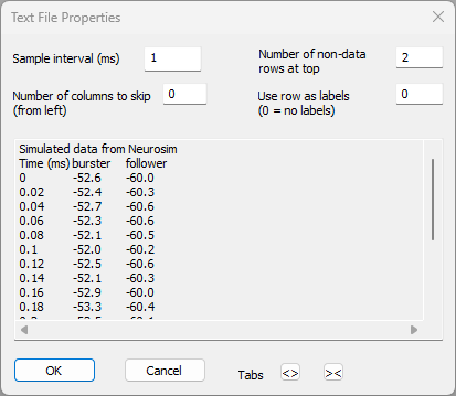
- Set the Sample interval to 0.02.
You have to tell Dataview what the sample interval is, since there is no consistent text file format that contains that information (although in this case the left-hand column contains the time stamp for each sample, so we can see the sample interval). - Set the Number of columns to skip to 1.
The left-hand column of this file contains the sample times. However, Dataview has no way of knowing this - it is just a column of numbers. Since we don't want to display the time as a trace, we instruct the program to skip the first column when reading data from the file. - Leave the number of rows to skip at 2.
The top two rows contains header information. Dataview detects any non-numeric values in the top row(s) and will pre-select these rows for skipping. However, if the top row contained numeric data that was not part of the recording (e.g. a date), you would have to adjust this parameter manually. - Set Use row as labels to 2.
The second row contains header text for the column below. These can be imported as trace labels. Any skipped rows not specified as trace labels will be incorporated into the file comment. - Click OK.
- The File information dialog displays - click OK to dismiss it.
- When the file loads, click the Show all timebase toolbar button (
 )
) - Hold down the control key and click the Autoscale traces toolbar button (
 ).
).
(If you do not hold down the control key, only the selected axis autoscales.)
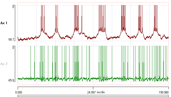
You should now see these data:
If you open multiple text files, Dataview will remember the settings supplied for the first file, and make these the defaults for the subsequent files.
Commercial formats
DataView currently works with Axon Instruments files in gap-free or episodic format (.abf), including the new version 10 format, Axograph files (axgx) with a simple format, CED Spike 2 files (.smr), CED Signal files (.cfs), EGAA ECR-mode files, EGAA scope-mode files, EDF (European Data Format) and EDF+ files (.edf), Wintrontech files (.vet), MultiChannel system files (.mcd), sound files (.wav), raw binary (.bin) and plain text (.asc, .txt or .csv) files.
Here are some details about how DataView handles specific features of various formats.
Multi-timebase recordings
Some commercial data acquisition systems allow you to sample data at different rates for different traces. In these situations DataView treats all traces as if recorded at the fastest sample rate within the record, with missing data points in the slower traces filled by linear interpolation. This means that certain analysis routines (e.g. spectral analysis) may yield inaccurate results with traces not recorded at the fastest sample rate.
DataView cannot currently handle formats where the timebase changes within a record.
CED Signal files
CED Signal files are frame based, where each frame is like a single sweep of an oscilloscope. When DataView opens these files, the frames are concatenated into a single continuous record, with the start of each frame marked by an event in channel a. The elapsed time of each frame is shown as an event tag label, along with any frame comment. The time is also stored in the variable value of the appropriate event, so that it can be easily copied into a spreadsheet such as Excel (see Listing Event Parameters below).
Files with gaps
Some commercial formats generate files with gaps in them indicating time sections in which acquisition was switched off (e.g. CED Spike files – see below). By default, DataView shows the gaps as zero-valued data which display in grey on the screen. You can hide the inactive data altogether by de-selecting the View: Show inactive data sections menu option. You can remove the gaps altogether with the File (or Transform): Concatenate gaps menu option. This re-writes the file as a native DataView file, and removes the gaps in the display and only shows regions in which all traces contain data. The start of each data section is marked with an event, and the event label gives the real time of the start of that section. The start time is also stored in the variable value of the appropriate event.
CED Spike files
Spike files may contain gaps within them (see above). Text marks in Spike files are imported as markers in DataView (see below), while ordinary markers are imported as events.
DataView can read event-only Spike files. It constructs a dummy 0-filled data trace.
DataView can read waveform Spike files. The waveforms are treated as if they were short sections of data with gaps between them.
Axon Instruments (Molecular Devices) files
DataView can read Axon Instrument files stored in either gap-free or episodic format. In the latter case, the episodes are concatenated into a single continuous record, with the start of each episode (sweep) marked by an event. The event label gives the real time of the start of that episode. The start time is also stored in the variable value of the appropriate event.
DataQ files
DataView uses the DataQ-supplied ActiveX control to read wdq files, and this only provides access to the data themselves and the engineering units applied to the data. Parameters such as user annotations, scales, cursors etc are not retrieved from the wdq file.
EDF+ files
EDF+ files can be either continuous or discontinuous. Discontinuous files are treated as frame based, where each data record is regarded as a separate frame and the gaps between frames are not shown (i.e. the data are concatenated) (see CED Signal files above). Time-stamped annotation lists (TALs) that occur within visible parts of the data (i.e. not in gaps between frames) are shown as labelled events.
MultiChannel System files
DataView can display MultiChannel System files using the Neuroshare library to read mcd files. The display is currently limited to continuous and triggered analog data with each trace recorded at the same sample rate. For triggered recordings the sweeps are concatenated one after another, with the start time of each sweep indicated as an event in channel ‘a’. The relative experimental time of the sweep (in seconds) is shown in the event labels, and stored in the event variable.Spike waveform fragments (segments) are not displayed, and nor are digital signals except for the trigger event mentioned.
User-defined files
As well as reading data from commercial acquisition files, you can also generate data externally as a text file, and import it as seen above, or you can use the built-in expression parser, or you can paste data from the clipboard.
Using the built-in expression parser
The built-in expression parser can be used to write a variety of arithmetic functions.
- Select the File: New: User-defined menu command to open the New file dialog box.
- Set the desired Sample interval and the Number of samples per trace. The defaults are suitable for this demonstration, so leave them.
- Enter the arithmetic expression that defines your data into the Equation edit box. By default it simply shows 0, which means that the file will contain 1000 samples all of value 0. This is probably not what you want.
A full description of the equation syntax is available here, or by pressing F1 to activate the built-in help.
Most functions are time-dependent. The algebraic value xt is used to indicate current time in the expression. Thus the expression sin(2*_pi*xt/360) will yield a sine curve with each millisecond equivalent to 1 degree of angle. (The expression sin(f*2*_pi*xt/1000) will generate a sine wave with the frequency f if you substitute the actual value of f into the expression; e.g. sin(50*2*_pi*xt/1000) generates a 50 Hz sine wave.)
You can include random numbers in your expression. The algebraic function rndu() generates a random number with a uniform distribution greater or equal to 0 and less than 1. The expression rndn() generates a random number with a normal (Gaussian) distribution, with a mean of 0 and a standard deviation of 1. To generate normal random variables with other parameters, simply add and multiply appropriately.
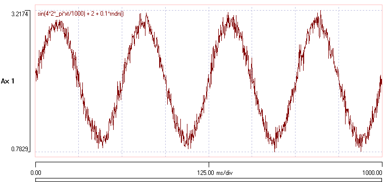
- Enter the expression sin(4*2*_pi*xt/1000) + 2 + 0.1*rndn() (you can cut-and-paste the expression in bold text from this web page if you wish).
- Click OK, and enter a file name when asked. After a brief pause, the new file should load.
- Click the Autoscale toolbar button.
You should now see a display containing a 4 Hz sine wave with additional random noise which has a mean of 2 and a standard deviation of 0.1 added to it.
Event-Only Files
You can construct event-only files by checking the Dummy data box in the New file dialog activated by the File: New: User-defined menu command. These files allow you to read in or generate events for timing analysis, but do not have any waveform data on construction.
Paste Data from the Clipboard
New file
You can generate a new file from data that have been constructed in an external programme and copied to the clipboard. There are two types of data that can be pasted: text format and Neurosim-specific format. The latter is a bespoke format generated by the separate simulation program Neurosim, while the former can be generated by any program that produces text output (typically, Excel). Text data can themselves be in two formats: contiguous and sparse.
Contiguous data
Contiguous data have values specified at fixed time intervals, with no missing values. The time interval itself is not read from the source, but is supplied by the user.
- Open the text link burst.txt in a new tab or window in your browser.
- Select all the text and copy it to the clipboard.
- In most browsers this can be done by pressing control-a, then control-c.
- Select the File: New: From clipboard: Contiguous data command.
- Proceed as described previously for text format files. Note that in this case, the first column specifies the time of each sample, and that these values are evenly spaced. This column should be skipped.
Sparse data
Sparse data are data collected at variable time intervals. In the table below, the left column (time) denotes the time (ms) into the recording at which the data were collected, while the tab-separated right column contains the data values at the specified times. (In this demonstration, both columns were constructed using random values, and the time values were then sorted into ascending order.) A similar table could be constructed in Excel or any text editor.
In the table there is just one data column and so there will be just one trace, but if there were multiple data columns then multiple traces would be constructed. But note that the datum in each trace is assumed to be collected at the single time specified in the left-hand column for that row. If you want to incorporate traces collected at different time intervals, you must paste the additional traces one-by-one using the Transform: Paste trace: Sparse data command (see below).
time value 37 -1.7266 84 2.1104 148 1.0697 161 0.4513 170 -2.7969 174 -1.0098 188 -0.6982 242 -0.1060 267 0.1238 395 -0.7872 416 0.9317 468 0.3044 470 1.6138 558 0.3223 628 0.1751 676 -0.7698 752 -0.2267 848 0.1580 914 0.2280
- Copy the table above to the clipboard by dragging across it and pressing control-c (or whatever your browser uses for copying).
- In DataView, select the File: New: From clipboard: Sparse data menu command to open the Paste New Spares File dialog.
- Note that the default Sample interval is 1 ms, and the Number of samples per trace is set to 992, which is enough to show all the data (the latest time is 991 ms, and time starts at 0). We will change from the defaults just to demonstrate what happens:
- Set the Sample interval to 0.5.
- Note that the Number of samples doubles, so all the data will still be shown.
- Set the Number of samples to 2001 to make the end display time have a more "roundedThe '1' at the end is because time starts at 0. So a time span of 0 - 1000 ms at 0.5 ms intervals requires 2001 samples." value.
- Check the Row above data contains trace labels box, to use the text "rnd sd 1" as a trace label.
You now have to decide how you want to fill in the gaps between the times at which data are specified. You can set the intervening data inactive, or you can fill the gaps by various interpolation schemes. For now, choose the former - we will see interpolation in action later (see below).
- Select Inactive gap.
- Click OK.
- Choose a name and location for the new file.
The new file should load, showing each datum as a dot on the display. The gaps are filled with grey zero-valued dots, showing inactive data.
- Toggle the View: Show/Hide: Inactive data sections off (no menu tick), to hide the grey dots.
- If you want, Save the file so that you can reload it later (it is used in the New trace: Sparse data tutorial below).
Continue the New trace: Sparse data tutorial below to see the various interpolation options in action.
New trace
You can also construct a new trace in an existing file from clipboard data using the Transform: Paste trace command. As with the New file option, data can be contiguous or sparse.
Contiguous data
The data can have a non-numeric text first line which will form the trace label, but the remaining text should be numbers. If there are more clipboard data than samples in the (existing) traces then excess data are discarded. If there are fewer data, then the remainder are either zero-filled or set inactive, depending on the user choice.
Sparse data
Sparse data are supplied in the same format as for a new file (above), except that only one trace can be pasted at a time into an existing file.
To see an example of this with real data, view the Display event parameters as data tutorial, but for now we will use the data from the table above.
- Reload the file you saved in the New file: Sparse data tutorial above.
- Copy the data from the table above onto the clipboard (if you have altered the clipboard contents since you last did this).
- Select the Transform: Paste trace: Sparse data menu command to open the Paste Sparse Trace dialog.
There are 4 options for interpolating the gaps between the defined points in the data; Linear, Cubic spline, Bezier, and PCHIPPCHIP stands for piecewise cubic hermite interpolating polynomial, which is why the acronym is commonly used!. To see each of these in action:
- Click the Show button under the list to activate the Interpolate Time Series dialog.
- This dialog is described in detail in the Interpolate time series: External data tutorial, but for now:
- Select each interpolation option in turn to see the resulting curves.
- Note that with these data the Bezier and PCHIP interpolation options produce quite similar results.
- Select the Linear option and then click OK to dismiss the dialog.
- Note that the Linear interpolation option is selected in the original Paste Sparse Trace dialog. Leave this be.
- Uncheck the Write new file checkbox.
- Click OK.
A new trace is written to the existing file. It is exactly the same as the first trace, except that the gaps between the specified data points are filled by linear interpolation, resulting in a jagged set of straight line segments.
- Repeat the Paste trace: Sparse data process, but this time select Cubic spline interpolation to fill the gaps.
This connects the specified data with a smooth curve. Note that curve projects considerably beyond the maximum and minimum of the specified values (note the axis scales, which autoscale automatically for the new trace).
- Finally, repeat the Paste, but select the Bezier option.
This smooths the gap fill data, but less aggressively than the cubic spline, so the line follows the data more closely. It is what is normally used by Excel to produce smooth connecting curves between points in and XY scatter graph
At this point, it may be useful to superimpose the traces to compare the interpolation methods more clearly.
- Select the Traces: Format menu command to open the Trace Format dialog box.
- Click the High X button to give the traces contrasting colours.
- You could choose the colours individually, but this is an easy shortcut.
- Set the Axis each of the 4 traces to 1, so that they all display on the same axis.
- Uncheck the Show box for Axes 2, 3 and 4.
- Click OK to dismiss the dialog.
- Select the Traces: Dot size: Medium menu command to enlarge the data dots.
- Click the Autoscale vertical () toolbar button.
At this point the display should look like this:

(available as the file sparse data).
Note that all 3 interpolation methods go through each actual data value from the source (the black dots). However, the cubic spline curve (blue), while the smoothest curve, shows large excursions above and below the actual data. The reason can be clearly seen with the 2 data points just before the middle of the display. These are close together and thus produce a steeply rising slope, which causes the cubic spline to project considerably above the upper point before dropping to meet the next point. This sort of extreme excursion is avoided with the Bezier and PCHIP interpolation methods (and is avoided completely with linear interpolation, in which there is no projection at all beyond the source data).
The properties of the various interpolation methods are explored in more detail in the Interpolate time series: External data tutorial.
Saving files
Original acquisition files
After you have made changes to a file you may want to save it. You CANNOT overwrite original data acquisition files (Axon, CED etc. files), and your options for saving depend upon the changes you have made. If you have only changed display settings or DataView-specific elements such as annotations or events, but have not changed the data themselves, then you can save the DataView specific elements in a header file.
- Select the File: Save command or press the keyboard shortcut (control s).
This will save an additional file with the same name and directory location as the source data file, but with the extension “dtvw-hdr”. This file contains the DataView specific elements, and by default it will be loaded when next the source data file is loaded.
If you make changes that affect the data themselves (using options from the Transform menu) then you will always be prompted for a new file in which to save the changed data. This file will be in the native DataView binary format (with the extension dtvw-dat). You can also explicitly save files into this format using the File: Save as menu command. This command also gives you the option to save the data themselves in text format.
Files that already exist in DataView format can be saved with their original filename using the File Save command, and this will overwrite the original (DataView format) file.
Extracting Sub-Sections of Files
The File: Extract sub-file menu command (also available on the Transform menu) allows you to extract a region of the file and write it as a separate file. This is useful for saving disk space and load time if only a small section of a long file contains useful data. An example is given here.
Active/Inactive Data Sections
If a file contains multiple sections of interest separated by regions of no interest, you can make the no-interest regions inactive. This means that no data are saved for these regions, which can substantially reduce file size. To do this you first have to identify the regions of interest by marking them with events (see below for methods). Then select the Transform: Events only active menu command. The advantage of this method over the Extract sub-file process is that the relative timing of the active regions is maintained within the file.
Writing Video (avi) Files
The File: Write video file(avi) menu command writes a scrolling display of the data into a video file. A walk-through is available here.
Writing Audio (wav) Files
The File: Write audio file (wav) menu command writes one or two (mono or stereo) traces into an uncompressed audio file in the standard wav format. You can write the whole source file, or just that section visible in the main display, and you can write with either 8-bit or 16-bit resolution. If you check the Normalize box in the Make Audio File dialog the largest peak-to-peak signal will play at full volume.