Spike Shape Analysis

A fairly common task in some fields in neuroscience is to characterise intracellular spike shape with specific numerical values representing features such as threshold voltage, width at half-height etc. The Analyse: Spike shape facility helps with this.

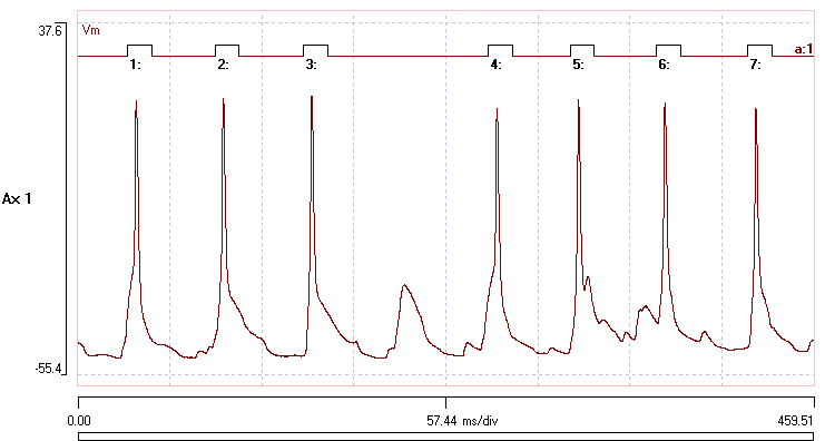
You have to start this with a data trace containing the spikes (obviously) and an event channel containing events that locate spikes, where each event encompasses the peak of a single spike. The exact timing does not matter, so long as the peak is within the eventThe simplest way to detect intracellular spikes is usually with the Event edit: Threshold facility, with high-pass pre-filtering if necessary to remove any big DC shifts..

• Open the file spike shape and note that channel a contains appropriate events.

• Select the Analyse: Spike shape menu command to display the Spike Shape Analysis dialog box. Note that the dialog can be resized by dragging on a corner.
• Set the Spike event chan to the appropriate value (the default a is correct in this case), and the Spike trace to the trace containing the spikes (again the default 1 is appropriate).
• Click Analyse.

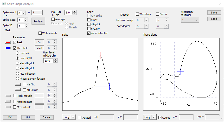
Within the dialog, the graph on the left shows the waveform profile of the spike from the event specified by the Spike ID, over the specified region of interest (RoI) on either side of the spike peak. So in this case we are looking at the waveform 8 ms on either side of the peak of the first spike in the recording. The graph on the right shows the phase plane of the spike (voltage on the X axis, rate of change of voltage (1st derivative) on the Y axis).

You can scan through each spike in the recording by clicking the up spin button of the Spike ID. You can also, of course, edit the ID value directly.

Mark features

The controls in the Mark panel specify what spike characteristics are marked and measured.

• Check and then un-check each box in turn in the Parameter list, to see the effect. Note that there is no post-spike trough in the waveform, and so the Peak-trough parameter cannot be determined.
• Click the List button to show the values associated with each feature in a Results dialog (you may need to click < > to expand the tab spacing to line up values in the dialog box).
• Note that the primary value of selected features is also written into the edit box beside check box.

If you check the Write events box then events will be written into the selected channels so as to mark the timing of the features in main view when you exit the dialog box by clicking OK (no events are written if you exit with Cancel). Note that the time and amplitude resolution of data values marked as events is limited to the sample values and intervals of the original recording. Data values shown with the List facility may be more accurate since intermediate values are calculated where appropriate by linear interpolation between samples.

The following features can be marked. If the feature cannot be detected, then no mark is made and -999 displays with the List command.

Peak

This marks the peak of the spike – the maximum voltage within the event specifying the spike.

Threshold

This estimates the spike threshold. For each threshold type, the time from the point at which the rising voltage crosses threshold to the time at which the falling voltage re-crosses the same threshold is marked.

Conceptually, threshold voltage is the “point of no return” at which the membrane potential takes off towards the spike peak, and although it can be defined absolutely in terms of membrane currents (Platkiewicz & Brette, 2010), it can only be estimated subjectively from the waveform profile. However, there are objective criteria which can be used to aid that estimation, although none of them are completely satisfactory for all types of spike profiles (Sekerli et al., 2004).

Voltage (User mV): The simple voltage threshold is the latest time before the spike peak at which the voltage crosses the user-specified value. You can specify the value either by directly editing the User level, or by clicking at an appropriate point in either graph. For this recording, a value of -26 mV gives a reasonable by-eye estimate of the threshold which works quite well for each spike in the recording.

Rate of rise (User dV/dt): The rate-of-rise threshold is the latest time before the maximum rate of rise at which the specified rate of rise is achieved. You can specify the value either by directly editing the User level, or by clicking at an appropriate point in either graph (in the Spike graph the rate of rise is set to the value at the time location clicked, rather than the voltage location). Note that clicking on the Spike graph may give unexpected results because there may be several locations on the spike waveform that have the same rate of rise. It is the latest before the maximum rate that will actually be marked.

Specifying the rate of rise is one of the standard ways of specifying threshold objectively. The default value of 10mV/ms works well for some spikes, but fails dismally for the 3rd and 5th in this recording.

Maximum 2^nd Derivative (Max d²V/dt²): Working back from the spike peak, the local maxima for the first, second and third derivative are successively identified, and that of the second derivative is taken as the threshold. If you use this you may need to smooth the waveform or derivative (see below), since higher derivatives are very susceptible to noise.

Maximum 3^rd Derivative (Max d³V/dt³): Working back from the spike peak, the local maxima for the first, second and third derivative are successively identified, and that of the third derivative is taken as the threshold. If you use this you may need to smooth the waveform or derivative (see below), since higher derivatives are very susceptible to noise.

The 3^rd derivative method provides a good “by eye” fit to what appears to be threshold for the spikes in this recording.

Rise inflection: When a spike is triggered by an EPSP or current injection, the waveform initially rises with a rate of rise that decreases with time (a classic RC charging curve). However, if the stimulus leads to a spike, the rate of rise starts to increase again, as the voltage dependent channels are activated. The time of this inflection, if it exists, is automatically detected. This method tends to work well for spikes elicited by current injection, but less well for spontaneous spikes or spikes generated by multiple EPSPs (as is the case in the sample recording).

Phase-plane inflection: This attempts to identify the point where the phase-plane graph starts to curve strongly upwards from the rest position, which presumably indicates an overall increase in inward current. It is Method II described by Sekerli et al. (2004), and reports the voltage at the peak of the second derivative with respect to voltage in the phase-plane, at a voltage below that of the maximum rising slope. It works well for some spike shapes, but, like all the other methods, less well for others!

The half-height width, which is the width at the voltage which is half way between the threshold and the peak, can be marked. Similarly, the 10%-90% rise time, which is the time delay from 10% above threshold to 90% above threshold (where the spike peak is 100%), can be marked.

Peak-trough

This marks from the peak to the first trough after the peak, if any trough is detected. In the sample file, only Spike 5 has a trough within the RoI (and this is caused by a following EPSP rather than a post-spike hyperpolarization).

Max rise

This marks the point at which the maximum rate of rise of the voltage (i.e. the peak of the first derivative) before the spike peak is achieved.

Max fall

This marks the point at which the maximum rate of fall of the voltage after the peak is achieved. In this case the time measurement is backwards to the same voltage on the rising phase.

A particular set of analysis parameters can be Saved to a configuration file and re-Loaded for subsequent analysis of other files if desired.

Average

Check the Average box to display the average of all spikes marked by events in the trace, rather than the individual spikes. By default, the registration point for averaging is the time of the Peak of each spike, but if you wish you can set this to be the time at which Threshold is crossed (see below for how to define threshold).

Noise reduction

If you have a lot of noise in the recording you can apply a Savitzky-Golay filter. Membrane noise can have a big effect on the derivative of the waveform, and since several analysis routines depend on this, noise reduction may be crucial.

• Check the Show: d³V/dt³ box to display the 3rd derivative of the waveform as a green trace superimposed on the raw waveform (note that this is scaled to have the same peak amplitude as the spike). Although the peak is quite clear, there is a substantial amount of noise in the derivative trace. Lower-order derivatives are also noisy, although less spectacularly-so.
• Check the Smooth: Waveform box. Note that the noise oscillations in the derivative waveform are substantially reduced.

Smoothing the waveform does reduce noise, but it is also effectively low-pass filtering and so can distort the spike shape, so smoothing should be kept to the minimum necessary The S-G filter has 2 user-specified parameters: the polynomial degree, and the number of samples in the window over which the polynomial is fitted. For a spike, a relatively high-order polynomial (degree 6) is probably best.

• You can check how much smoothing affects the waveform by checking the Show: Raw spike box. This shows the unsmoothed waveform as a red trace superimposed on the smoothed waveform. At the default setting there is virtually no visible change in the spike waveform, which is what you want
• To see the effect of excess smoothing, increase the half-window sample to 60, and note that large deviation of the smoothed waveform from the red trace. Then return to a value of 6. At this level, the smoothed trace is almost identical to, and superimposed over, the raw trace, so the latter is barely visible.

Derivative calculation

The voltage derivatives can be calculated either using a fourth-order finite difference method (the default), or using a Savitzky-Golay filter. The latter automatically applies smoothing to the derivatives.

• Uncheck the Smooth: Waveform box
• Check the Smooth: Derivatives box

Note that you can apply smoothing to both the waveform and the derivatives if you wish – the waveform smoothing is done first, and then the smoothed derivatives are calculated from the smoothed waveform.

Sample rate upscaling

If a data file is recorded at a relatively low sample rate, the waveform in the “join the dots” standard display may not show the shape of the spikes accurately.

• Close the Spike Shape Analysis dialog box (it is modal, and you cannot do anything else in DataView with it open).
• Open the file spike shape undersample.

The ADC sample rate for this file was 10 KHz, which definitely meets the Nyquist criterion for the data, but does not provide a good "join the dots" display - the first spike apparently has a lower peak amplitude than the second spike.

• Re-open the Spike Shape Analysis dialog box.
• Click Analyse.
• To see the spike shape more clearly, set the Max RoI (maximum region of interest) to 1 ms. (These spikes are very brief, and this still encompasses the key features.)

The peak of the spike is clearly truncated, and the jagged phase-plane graph reflects the paucity of data points within the spike itself.

• Note the measured peak amplitude of the first spike, which is 24.7 mV.
• Advance the Spike ID to 2 to look at the second spike. The spike appears less truncated, and Its peak amplitude is 30.7 mV, which is significantly larger than that of the first spike.

So long as the Nyquist criterion has been met, the apparent data sample rate can be increased by interpolation using the FFT technique.

• Re-set the Spike ID to 1 to return to viewing the first spike.
• Select 8 from the the Frequency multiplier drop-down list.

The spike now has a more realistic shape, and its peak amplitude is now 30.8 mV. The interpolated waveform (black trace) is slightly delayed relative to the raw data (red trace), but its width and general shape appears undistorted. The phase-plane graph is now smooth.

• Advance the Spike ID to 2 to look at the second spike using the frequency multiplier.

The measured peak amplitude of the second spike is slightly increased (to 31.6 mV), but now the two spikes have peak amplitudes that are very similar. The apparent difference in amplitude in the raw data is due to the A-D converter not acquiring a sample at the exact time of the peak of the first spike, but nearly doing so for the second spike.

Frequency upscaling should be used with care since it can introduce spurious oscillations in the flatter portions of the waveform (the Gibbs effect), although this has been minimized by applying a window which tapers to zero on either side of the region of interest. Better results may be obtained by using the Transform: Increase frequency option on the whole file. This works purely in the time domain, and artefactual oscillations are limited to the start and end of the data file as a whole (rather than just the spike window as is the case here). However, this obviously produces a proportionally larger file.

 

---