Filter Data

Principles

First I acknowledge my debt to the excellent (and free!) book “The Scientists and Engineers Guide to Digital Signal Processing” by S. W. Smith. Much of the following is a digest of what I have learned from this source – although I offer no guarantees that I have completely understood the many issues involved!

All digital filters have an impulse response, a step response, and a frequency response. The impulse response is the output when presented with an input that consists entirely of zeros except for a single non-zero sample. The step response is the output when presented with an input which steps suddenly from a constant signal of one value (usually zero) to a constant signal of some other value (usually 1). The frequency response is a graph of the filter gain (output-to-input ratio) plotted against the frequency of the signal. Each of these three characteristics completely describes the filter – if you know one, you can, in theory at least, calculate either of the other two by various mathematical techniques.  The file impulse contains an input signal consisting of an impulse followed by a step, while the file sin-100-20-5 contains a mixed sine wave signal with frequencies of 100, 20 and 5 Hz. These two files can be used to investigate the responses of various filters.

Nyquist frequency

A crucial point about digital filters is that they can only perform operations at frequencies up to the Nyquist frequency of the data (half the sample frequency). Furthermore, the original analogue data should have been filtered to remove any components with a frequency higher than this prior to being digitized, or the dreaded aliasing will occur, in which the high-frequency signal fraudulently appears within the low-frequency data.

There is a separate tutorial on the Nyquist frequency and acquisition sample rates.

Filter domain

Before filtering any signal it is important to consider how information is contained within that signal. In particular, one should know whether it is the amplitude at particular times that contains the information (time domain signals), or the frequency at particular times that contains the information (frequency domain signals). The reason that this is important is that different types of filter are appropriate for different types of signal, and a filter that is optimized for performance in one domain will inevitably perform badly in the other. This seems to be one aspect of that general rule of the universe with which we are all horribly familiar, namely, there is no such thing as a free lunch.

A typical frequency domain signal is an audio signal. A single digitized data point containing the amplitude of the sound pressure at a particular moment in time is of very little interest, what matters is the relationship of this data point to the others around it, which tells us about its frequency (pitch) and the amplitude of the sound as a whole. In contrast, a typical time domain signal (in a neurophysiological context) would be an intracellular recording. In this case, the amplitude of the signal at any particular moment represents the membrane potential of the neuron at that moment, and that may be of very great interest. However, some neurophysiological signals do contain information in the frequency rather than the time domain, such as an EEG recording, where the various rhythms (alpha, gamma etc), contain the information.

Filters that are optimized for signals in the frequency domain are best characterized by their frequency response. The purpose of these filters is to allow some frequencies of signal to pass, and to block other frequencies. It is possible to design filters that have extremely sharp cut-off frequencies, so that they can separate out very similar frequencies within the signal. The penalty for this is considerable overshoot or “ringing” in the step response. So long as the data have been pre-filtered to the Nyquist frequency this does not matter, since the digital filter would then never see a real step response. However, not many data acquisition systems perform such pre-filtering automatically, and thus step inputs (such as a current pulse, or voltage clamp step) are frequently recorded unfiltered. If this step is then passed through a digital filter, the output gets very distorted. In contrast, filters optimized for signals in the time domain usually have a very smooth step response, so that they produce little amplitude distortion, but have a relatively poor ability to discriminate between different frequencies within the signal.

Edge effects

Most digital filters produce distorted output at the beginning and end of the section of filtered data. The length of distorted data depends on the filter settings, but you should treat these edges with caution (preferably by not using them in any analysis).

Frequency domain

FIR

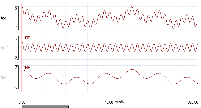
• Open the file sin-100-20-5. The trace shows a waveform containing a mixture of sine waves, and was constructed using the Excel spreadsheet program. The frequency components are 100 Hz, 20 Hz and 5 Hz.
• Select the FIR filter optionFIR stands for finite impulse response: a type of filter whose response to an impulse signal eventually settles to zero. Another class of filters have an infinite impulse response (IIR) and their response to an impulse never settles to zero. from the Transform: Filter menu.
• Set the lower cut-off to 50 and the upper cut-off to 500 (note that the sample rate was 1000 Hz, and the filter frequencies cannot be more than the Nyquist frequency, which is half the sample rate). The default band pass option means that with these settings the filter will pass frequencies that are greater than 50 Hz, so the 100 Hz component of the signal should survive, while the lower frequencies should be removed.
• Click the Preview button at the bottom-right of the filter dialog.
  • In the Preview dialog, click the expand timebase toolbar button () twice. You should see that only the high frequency component of the signal passes the filter. The signal distortions at the start and end of the preview are edge-effects as the filter settles.
• Select the Band stop option in the main dialog, and note in the preview how the high frequency component is now eliminated, and the middle- and low-frequency components survive.
• Click OK to write a new file with the filtered data added as a new trace.
• Repeat the filter process, but this time stay with the Band pass option, and de-select Write new file before clicking OK.

The filtered data file should now look like this:

To check FIR performance in the time domain:

• Open the file impulse.
• Apply the FIR filter with 50-500 Hz limits and observe the Preview with Band-pass and Band-stop configurations. Note that there is considerable "ringing" in the filter output at the stepThe filter "assumes" that the sampling rate meets the Nyquist criterion, and the only way to get a step change in such a digital signal is if the original analogue signal oscillated at the moment of transition. transitions in the input signal. No need to actually apply the filter, unless you want to.

Time domain

RC-type

The simplest filter appropriate for the time domain is an RC-type. This is a recursiveA recursive filter re-uses part of its output as its input. filter and is the digital equivalent to an analogue single-pole resistor-capacitor filter. This is ideal for tasks like removing DC or long-term voltage trends from records, or smoothing sharp steps. DataView supplies both a low-pass and high-pass version of the RC-type filter.

• Open the file impulse.
• Select the Transform: Filter: RC-type menu command.
• Set the time constant to 50 ms.
  You can specify the filter parameters either as a time constant, or as a frequency. The time constant specifies the rate of exponential change in the output in response to a step change in the input, while the frequency specifies the –3 dB cutoff frequency (the frequency where the power of the output/input ratio is 0.5). The two parameters interact in a manner determined by the sample frequency.
• Click the Preview button and note the appearance of the filtered trace.
• Select the Bi-directional check box and note the change in the preview.
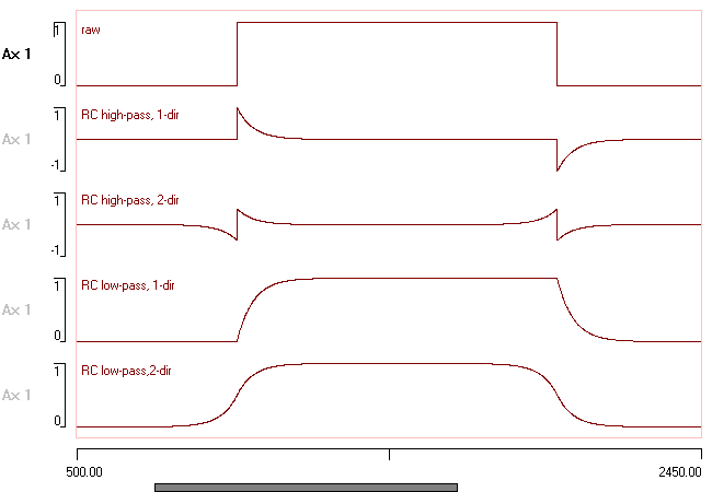
  This passes the data through the filter twice - once in the forward direction, and then backwards. It gives the filter a zero phase response, which is hard to explain without getting very technical, but the effect is easy to observe in the preview.
• Check the Low pass option in the main dialog, and again observe the effect in the preview.

The output from the various options applied to a square pulse is shown below:

Smoothing

Smoothing filters all work by replacing each data point by a value that is representative of the general values in a time window around that point. In DataView, these filters are all acausal, meaning that the window includes data points ahead of the point of interest, as well as behind it. All smoothing filters are low-pass filters.

Dataview provides several different types of smoothing filters, and they are all available through a single dialog interface with optional preview. This means that you can switch between different types and immediately see their performance. This is useful because, beyond some broad generalizations, it is often difficult to predict from first principles which filter type or parameter set will provide optimum performance for a particular recording.

Moving average

The simplest smoothing is the moving average filter, which replaces each data point by the average of itself and a user-determined number of data points on either side of the central point. The moving average filter is (or so I have read) the theoretical best filter for solving a common problem; the reduction of random white noise while keeping the sharpest possible step response.

Four types of moving average filters are available:

1. The standard flat (boxcar or top-hat) filter gives equal weighting to all data points within the averaging window. The interface allows you to specify multiple passes of the filter. Two passes approximates to filtering with a triangular kernel, while 4 or more passes approximates to Gaussian filtering (see below).
2. The moving median filter is the same as the moving average, except that it uses the median rather than the average (mean). Computing the moving median is more expensive than the moving average, and is not so efficient at removing random noise unless the noise is precisely normally distributed, but it is very much less sensitive to large but brief outliers (data “glitches”), which can distort the average and pull it in their direction.
3. The moving percentile filter is like the moving median filter, except that it allows the user to specify any percentile (0-100) of the data within the moving window as the replacement value. The moving median filter is actually a sub-set of the moving percentile filter, with the percentile specified as 50.
   The code for the moving percentile calculation is adapted from that supplied to me by Leemon Baird, who I gratefully acknowledge.
4. The Gaussian filter option applies Gaussian weighting directly – data points distant from the central point have a reduced weighting in the average, with the reduction following a bell-shaped curve on either side of the centre. A Gaussian moving average filter has similar properties to an RC low-pass filter. Note that specifying 4 iterations of a boxcar filter produces output similar to Gaussian filtering, and is usually considerably faster.

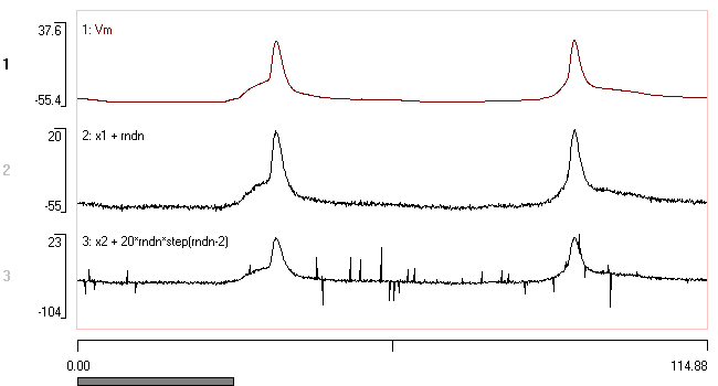
• Open the file spikes plus noise.

Moving average option

• Select the Transform: Filter: Smooth: Moving average menu command to show the Smoothing dialog, with the standard Moving average smoothing option pre-selected.
• Set the Trace to process to 2.
• Click the Preview button.
  The filtered data (lower red trace) are clearly much smoother than the raw data (upper black trace). However:
  • check the Superimpose box in the Preview window to compare the filtered and raw data on the same axis.
    The spike peaks have been considerably reduced in the filtered trace.
    
• In the main dialog, repeatedly click the down spin button of the Half window Samples control to reduce its value to 1 (giving a Time of 0.1 ms, since the sample interval of the recording is 0.1 ms). Note the spike and noise level in the Preview as you reduce the window.
• Set the Iterations to 4.
• In the Preview window, set the Start time to 25 and the Sweep duration to 20. This "zooms in" on the first spike so you can see the filter effects more clearly.

These parameters produces a reasonably smooth membrane potential trace without significantly reducing the peaks of the spikes. It seems to be close to an optimal setting for these data.

Moving median option

• Zoom out by clicking the compress timebase button () in the preview toolbar (or set the Sweep duration to 40).
• Change the Trace to process to 3. This is the trace with the outlier glitches.
• Uncheck the Superimpose box in the Preview window. The data glitches clearly distort the trace smoothed by moving average.
• Select Moving median to change to the robust form of the procedure.

It is apparent that the moving median filter does a much better job of retrieving the original recording than the moving average when there are outlier spikes in the data.

• Return the Trace to process to 2, and note the waveform in the preview.
• Return the filter to Moving average.

In the absence of the outlier spikes, the moving average is definitely superior to the moving median.

Gaussian

• With trace 2 still set as the trace to process, select Gaussian as the filter option.
• Change the -3 dB cutoff frequency to 500.
  The preview shows very similar results to the 4-pass moving average seen earlier. However, Gaussian smoothing is computationally more complex, and would probably be slower if filtering a long recording.
  (Note the distortion at the beginning and end of the preview trace, which are the "edge effects" mentioned previously. They do not occur in the moving average because the algorithm is different.)
• Just for completeness, switch the Trace to process to back to 3, and note that the glitches again perturb the output.

Robust LOWESS

The robust LOWESSLOWESS = LOcally WEighted Scatterplot Smoothing. smoothing technique is more sophisticated than the moving median because it attempts to identify outliers and distinguishes between these and genuine data peaks. The algorithm for LOWESS smoothing is described in the Robust fitting and smoothing section.

There are 4 parameters that control the process. The polynomial degree is set depending on how ‘bendy’ the expected best fit will be. It is rarely useful to set the degree higher than cubic. A degree of 0 means that a weighted moving average is used. The half-window width largely determines the degree of smoothing. Larger windows produce smoother output, but at the expense of loss of detail in following small but real trends in the data. The iteration number determines how many iterations are carried out in the outlier reduction process. A value of 0 means that no outlier reduction is carried out. The outlier threshold determines how far the data have to deviate from the median to be regarded as outliers.

• Set the Trace to process to 3, the Half window Samples to 2 and the Iterations to 2 and the Type to Moving average.
• Select Robust LOWESS as the smoothing Type.
  The preview shows a very glitchy output!
• Repeatedly click the up spin button of the Samples, until you reach 10. At this point the glitches have almost entirely disappeared from the filtered data.
  • Check the Superimpose box in the preview.

The LOWESS procedure does a good job of both reducing standard membrane noise and removing outlier glitches, while at the same time having little effect on the spike peak amplitude.

Savitzky-Golay

Savitzky-Golay (S-G) smoothing can be tuned to follow narrow peaks and troughs in the data more closely than moving average smoothing, but at the expense of less effective smoothing of slowly-changing data. It's also a lot slower. It works by taking a window of data on either side of a central point, and fitting a polynomial function to these data. The central point is then replaced by the value of the function at that location. The window then slides one sample forward in the recording, and the process is repeated. The user specifies both the size of the window, and the degree of the polynomial. Degree values of 2, 4 or 6 are normal, and the higher the order, the more closely the smoothed data follow peaks and troughs. The size of the window determines the overall amount of smoothing (just as in moving average smoothing).

An important potential advantage of the Savitzky-Golay filter is that it directly gives the derivative of the smoothed waveform, since this is available analytically from the polynomial function. Derivatives are notoriously susceptible to noise, and if you want to calculate the derivative of a membrane potential change it is common to have to smooth the data first (see e.g. the Spike shape tutorial). The Savitzky-Golay filter does both jobs in one go - although here we are only considering the smoothing aspect.

• Select Savitzky-Golay as the smoothing Type.
• If you still have trace 3 selected as the Trace to process, change it to trace 2.
  The S-G filter is not a good choice for glitch removal - its key advantage is its ability to follow suddent changes in the signal.
• Set the Polynomial degree to 6 and the Half window Samples to 10 (the latter might already be set from the LOWESS example).
• Check and un-check the Preview Superimpose box.
  The S-G filter reduces membrane noise with virtually no effect on spike amplitude or shape.

The “best” parameter settings for S-G smoothing will depend on the features of the data that you wish to preserve. As can be seen above, the parameters can be interactively hand-tuned using the transform preview facility.

So far we have looked at data where artificial noise has been added. What about the real recording?

• Set the Trace to process to 1.
• Check the Superimpose box in the Preview.

At the normal gain, the raw and filtered traces look virtually identical. However, if we zoom in we can see a difference.

• Set the Preview Start time to 50 and the Sweep duration to 15.
• Set the Preview top scale to -47 and the bottom scale to -51.

The trace was very "clean" to begin with, but there was still membrane noise that has been reduced by the S-G filter. If we were calculating a derivative, particularly a higher-order derivative, even a small amount of noise gets massively amplified, and the S-G filter can be very useful in reducing the problem. This is explored further in the tutorial on Spike shape analysis.

Narrow-band (notch)

Narrow-band filters either stop or pass a very narrow range of frequency. In the Dataview implementation, the bandwidth is about 0.0003 of the sampling frequency.

Narrow band stop filters are sometimes used to remove mains interference from a signal when they are configured in band-stop mode (a notch filter). However, this is usually not as efficient as the de-buzz technique described elsewhere because mains interference frequently contains harmonics at multiples of the base, and these are not touched by a narrow-band filter.

• Load the file notch test.

The lower trace shows a low-amplitude sine wave which has been constructed using a formula which generates a period of 60 ms, and hence a frequency of 16.66+ Hz. The upper trace shows the same sine wave embedded in noise with a standard Gaussian distribution. You probably wouldn’t be certain just by looking at it that there was any sine wave component in the upper trace because the signal-to-noise ratio is rather low.

• Select the Transform: Filter: Narrow band menu command to show the Narrow band filter dialog.
• Leave the Trace to process as 1.
• Set the Centre frequency to 16.667.
• Select the Band pass option.
• Click the Preview button.

The Preview window shows an edge effect at the start of the transformed trace (lower, red), but then the trace stabilizes to show the sine wave embedded in the original noisy trace (upper, black).

If you selected Band stop as the filter option, the transformed trace would appear virtually identical to the untransformed trace. However, the sine wave would be removed. This could be confirmed by activating the filter (by clicking OK), and then using the Analyse: Power spectrum facility (there is a tutorial on that here).

De-buzz

The specialized de-buzz filter to remove mains interference is described here.