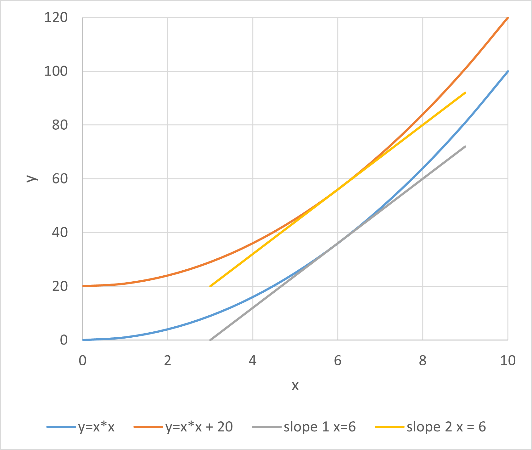
The slope of the y line at x = 6 is 12 for both equations, and is shown as the tangent.
To use the Hodgkin-Huxley model requires "solving" (aka integrating) 4 differential equations (22-25), i.e. equations where you know the rate of change of a parameter (its derivative), but you don't know its actual value. How do you do that?
In principle, there are two possible approaches: analytical and numerical.
We will start with two very simple equations:
\begin{align}
y &= x^2 \label{eq:eqYXX0} \\[1.5ex]
y &= x^2 + 20 \label{eq:eqYXX20}
\end{align}
If we plot these we get:
The curves are identical in shape, but the second is displaced 20 points above the first (as is obvious from the equations).
ElementaryElementary in the sense that it is one of the first things taught in a calculus course. But if you have not done any calculus it is by no means obvious intuitively, and you just have to take it on trust. calculus tells us that the slope of both lines (derivative of y with respect to x) at any value of x is 2x:
\begin{equation}
\frac{dy}{dx} = 2x
\label{eq:eqDerivYXX}
\end{equation}
Note that the 20 in the equation \eqref{eq:eqYXX20} just disappears in the derivative equation \eqref{eq:eqDerivYXX}. This is because the slopes of the 2 equations are identical at all values of x, it is just that one line is displaced vertically compared to the other.
Now, imagine that we know the derivative equation \eqref{eq:eqDerivYXX}, but do not know the original equation from which it came. How can we find the value of y for a given x? For a simple equation like this, there is a defined anti-derivativeAlso called the indefinite integral. which nearly gets us back to the original equation. In maths notation:
\begin{equation}
\int{2x\, dx} = x^2
+ C\label{eq:eqAntiDerivYXX}
\end{equation}
I said "nearly" because C is an unknown quantity and indicates that if all we have is the derivative, we do not know the vertical position of the line, we just know its shape. So the solution of \eqref{eq:eqAntiDerivYXX} could be either equation \eqref{eq:eqYXX0} or \eqref{eq:eqYXX20}. However, if we know the actual value of just one x, y pair, then we can figure out the value of C and locate the line in its vertical position. So if our known pair is x = 6, y = 56 we know that we are dealing with the second equation \eqref{eq:eqYXX20} and C = 20. But the pair is x = 6, y = 36, we are dealing with the first equation\eqref{eq:eqYXX0} and C = 0. The requirement for a known starting pair makes this an initial value problem.
The equation \eqref{eq:eqAntiDerivYXX} is an analytical solution to the differential equation \eqref{eq:eqDerivYXX}, and the joy of an analytical solution is that if we have the initial values, then we can jump immediately to find the exact value of y for any x. So if y = 3.2 when x = 0 and we know the derivative equation \eqref{eq:eqDerivYXX}, then we know that when x = 9.45 then y = 92.5.
HOWEVER: there are many derivative equations which have no known analytical anti-derivative, and this includes the four equations needed to use the HH model. For these equations we have to use a technique called numerical analysis to get a soluton.
If you know the value of y at a particular x (the initial values) and you know the slope of the line (dy/dx) at that point (which is a tangent to the curve), then you can estimate the value of y at a slightly bigger x (x + \(\Delta\)x) just by moving along the line a horizontal distance \(\Delta\)x and calculating the new y at x +\(\boldsymbol{\Delta}\)x from the linear tangent slope at the original x.
To put this more formally:
So to find the value of y at some value of x at a long distance from the initial value, you have to start with the initial values of x and y, and then "creep up" on the new value of x in small steps of size \(\Delta\)x, changing the value of y by \(\Delta\)y at each step.
This is the forward Euler method of numerical integration.
HOWEVER, this assumes that the slope of the line does not change between x and x + \(\Delta\)x (it uses the slope at x to make a linear projection to x + \(\Delta\)x). The problem is that the line is a curve, and its slope will change between x and x + \(\Delta\)x. The problem can mitigated by making \(\Delta\)x very small so that the curvature over the \(\Delta\)x distance has minimal effect, but this means that you only creep up on the new value in very small steps, which can take a long time. And even then, the problem does not go away, it just reduces the error.
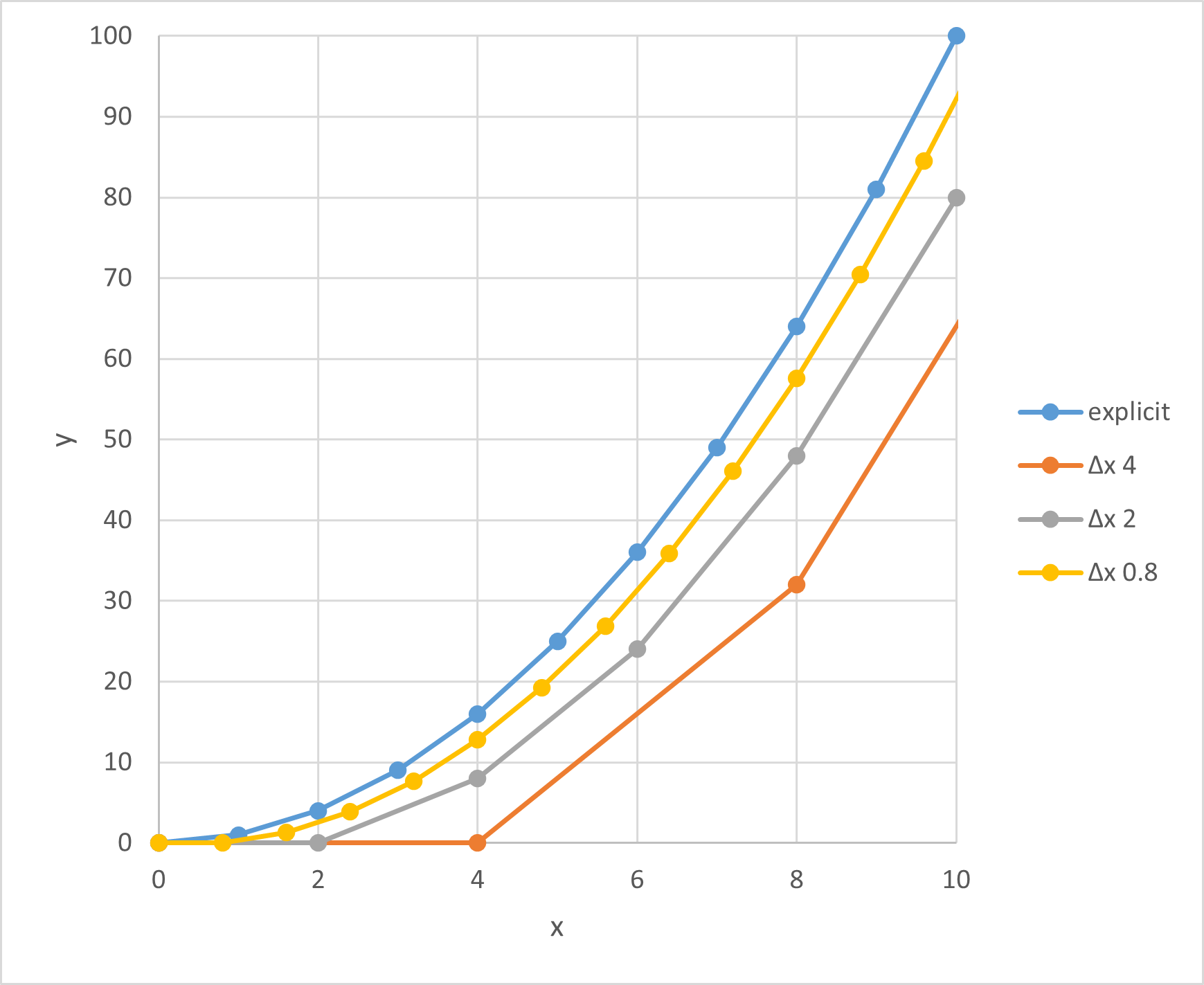
It is worth following through the most inaccurate plot when \(\Delta\)x = 4 (a ridiculously large step size for this equation domain).
If you want to explore this yourself, the Euler basic worksheet in the Excel tutorial allows you to see the effect of changing ∆x (named Xstep in the file) when integrating equation \eqref{eq:eqDerivYXX} with the Euler method. The key spreadsheet formulae are shown below:
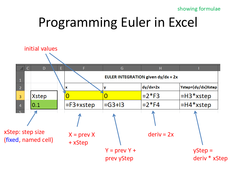
Fig. 11: Points of interest:
Clever mathematicians have come up with lots of improvementsThe "workhorse" method with a good compromise between speed and accuracy delights in the name of 4th order Runge-Kutta. on the forward Euler scheme that produce greater accuracy for the same step size, but forward Euler is easy to implement in Excel, and is satisfactory for our purposes so long as we keep the step size small.