a

b
c
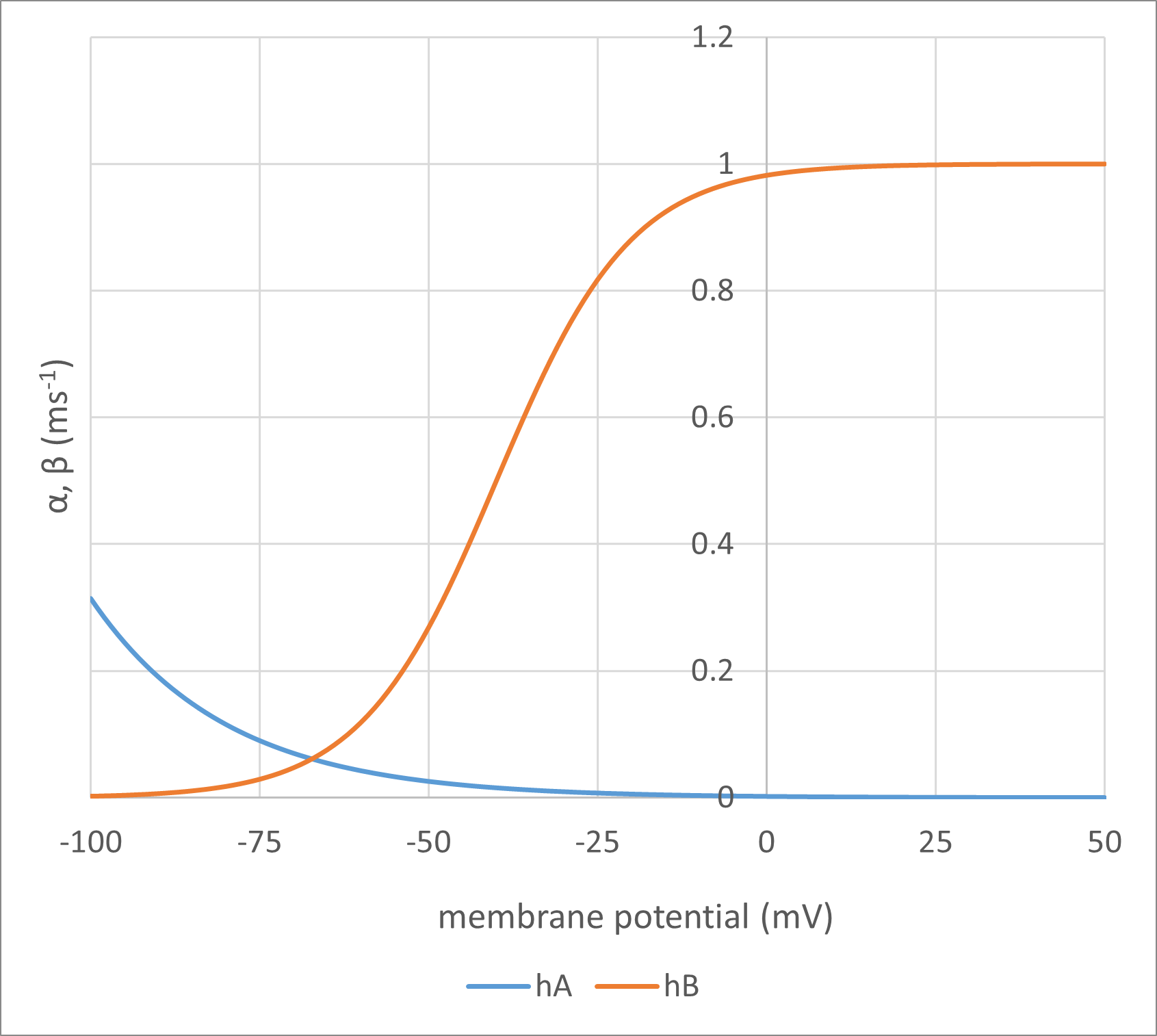
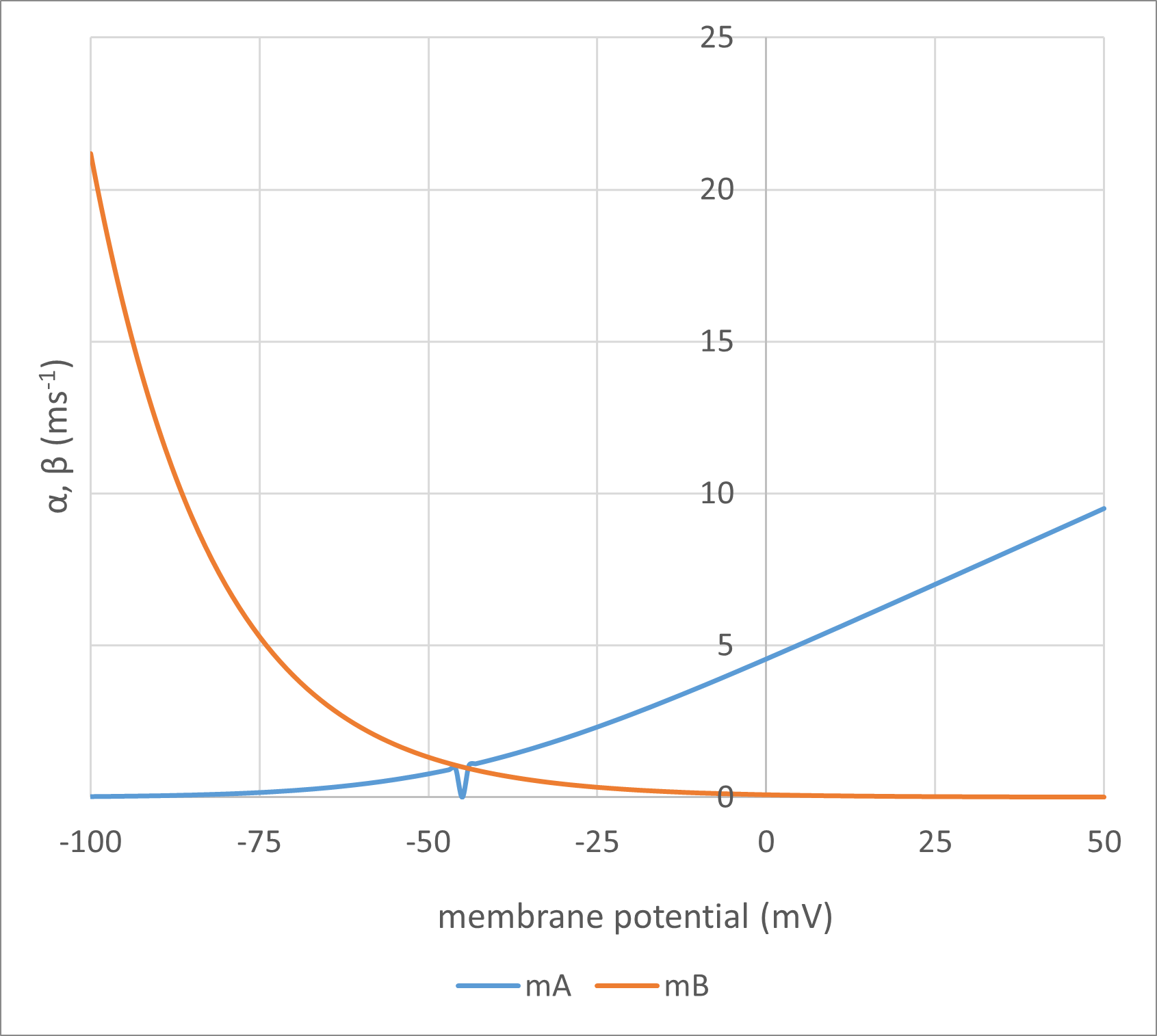
The HH formula for the opening transition rate constant \(\boldsymbol{\alpha}\) for the m gate in a Na channel is:
\[{\large \alpha_{m}} = \frac{\small{-0.1(V_{m}+45)}}{ e^ {\Large {\frac{V_{m}+45}{-10}}} \small{-1}}\]
If mV = -45 then:
\begin{align*}
{\large \alpha_{m}} &= \frac{\small{-0.1(-45+45)}}{ e^ {\Large {\frac{-45+45}{-10}}} \small{-1}}\\ \\
&= \frac{\small{-0.1(0)}}{ e^ {\Large {\frac{0}{-10}}} \small{-1}}\\ \\
&= \frac{0}{ e^ 0 \small{-1}}\\ \\
\end{align*}
Since x0 = 1 for any x,
\begin{align*}
{\large \alpha_{m}} &= \frac{0}{ 1-1}\qquad\qquad\\ \\
&= \frac{0}{0}
\end{align*}
hence a divide-by-zero error.
If we start with this formula:
\begin{equation*} \frac{dP}{dt} =\alpha (1-P) - \beta P \end{equation*}
We will first describe how a very simple set of basic assumptions about the gates leads to a series of equations that describe the active properties of the nerve membrane. We will then show how experimental data was used to provide numerical parameters to plug into these equations. Finally, we will show how the equations can reconstruct an action potential. We will use Excel spreadsheet formulae for all calculations.
In the HH model the individual gates act like a first order chemical reaction with two states. This can be written thus:
\begin{equation} \ce{shut <-->[\large\alpha][\large\beta] open} \label{eq:eqAlphaBeta} \end{equation}
The factors \(\boldsymbol{\alpha}\) and \(\boldsymbol{\beta}\) are the transition rate constants. The gate switches between states randomly, but \(\boldsymbol{\alpha}\) is the average number of times per second that a gate which is in the shut state opens, while \(\boldsymbol{\beta}\) is the average number of times per second that a gate which is in the open state shuts. At any moment in time all the gates within a particular class (m, h or n in Fig. 2) have the same value of \(\boldsymbol{\alpha}\) and the same value of \(\boldsymbol{\beta}\) (which is likely to be different from the value of \(\boldsymbol{\alpha}\)), but gates which belong to different classes may have different values of \(\boldsymbol{\alpha}\) and \(\boldsymbol{\beta}\). This gives the different classes their different properties.
The KEY FACTOR in the HH model which allows action potentials to be generated is that \(\boldsymbol{\alpha}\) and \(\boldsymbol{\beta}\) are voltage dependent.
It can be difficult to conceptualize the consequences of changes in the values \(\boldsymbol{\alpha}\) and \(\boldsymbol{\beta}\), so let us consider a very simple membrane system and follow through the logic.
Imagine a channel with a single activation gate in it, and when the gate (and hence channel) is open it has a conductance of 1 pSReal ion channels have a single-channel conductance in the range 2 - 200 pS depending on the type, but assuming a value of 1 keeps things simple. (10-12 S). Imagine the membrane has 1 million such channels, so that if all of them are open the total channel conductance is 1 µS (10-6 S).
Imagine that the membrane is at the resting potential and \(\boldsymbol{\alpha}\) and \(\boldsymbol{\beta}\) both have a value of 1. This means that on average, a gate (and hence channel, since there is 1 gate per channel) will spend 1 s in the shut state before it opens, and then 1 s in the open state before it shuts. In other words, over a period of time it will flicker between the open and shut states, but spend half that time open, and half that time shut. If follows that for the membrane as a whole, with 1 million such channels, at any point in time on average half the channels will be open and half will be shut, so the total membrane conductance will be 0.5 µS, i.e. half the maximum possible conductance. Since the individual channels open and shut probabalistically there will be some noise in this conductance value, but taking the average over a million channels makes the noise negligable. A formal definition of this steady-state open probability will be derived later.
Now imagine that there is a step depolarization of the membrane and that \(\boldsymbol{\alpha}\) instantly becomes 9, but \(\boldsymbol{\beta}\) remains at 1. Now a shut channel will only spend 1/9th s in the shut state before it opens, but it will still spend 1 s in the open state before it shuts. In other words it will spend 9 times longer in the open than shut state, so at any moment in time, 90% of the channels will be open and the total membrane conductance will be 0.9 µS. However, at the moment that the voltage changes, half the channels are shut, and on average they will be "stuckThe dwell time of the channel state actually follows an exponential distribution, so some channels will open almost instantly, others will take a relatively long time (and some may never open). But the average will be 1/9th s." shut for 1/9th s before they open. So even though \(\boldsymbol{\alpha}\) and \(\boldsymbol{\beta}\) changed instantly with the voltage change, the total membrane conductance does not instantly switch to 0.9 µS because the shut channels will take some time before they respond to the voltage change. Instead, the total membrane conductance "climbs" to its new value over a relatively long period of time. The rate of climb can be characterized by a "time constant" (\(\boldsymbol{\tau}\)), which will be quantified later.
Now imagine a similar set of channels but with gates where \(\boldsymbol{\alpha}\) and \(\boldsymbol{\beta}\) both have a value of 10 at the resting potential. The gates will flicker open and shut more rapidly than in the slow channel, but they will still spend equal time in the open and shut state, so on average at any moment in time half the channels will be open and half shut, and the total membrane conductance will be 0.5 µS, just as it was with the slow gates.
Now imagine that the step depolarization instantly switches \(\boldsymbol{\alpha}\) to 90, while \(\boldsymbol{\beta}\) remains at 10. By the same logic as before, the total membrane conductance will become 0.9 µS, which is the same as with the slow gates. However, at the moment of the voltage change, the shut channels now only remain stuck shut for an average of 1/90th s, rather than 1/9th. So the new overall conductance will be established much more rapidly than with the slow gates, i.e. the time constant of the conductance change will be shorter.
Here is a table showing the equations defining the voltage dependency that HH used in their model:
\begin{equation} \textsf{Table 1: Equations for the voltage dependency of }\alpha \textsf{ and } \beta\label{eq:eqAlphaBetaVoltDep} \end{equation}
| Na Activation (m) | Na Inactivation (h) | K Activation (n) |
|---|---|---|
| \[{\large \alpha_{m}} = \frac{\small{-0.1(V_{m}+45)}}{ e^ {\Large {\frac{V_{m}+45}{-10}}} \small{-1}}\] | \[{\large \alpha_{h}} = 0.07 e ^ {\Large {\frac{V_{m}+70}{-20}}} \] | \[{\large \alpha_{n}} = \frac{\small{-0.01(V_{m}+60)}}{ e^ {\Large {\frac{V_{m}+60}{-10}}} \small{-1}}\] |
| \[ {\large\beta_{m}} = 4 e ^ {\Large {\frac{V_{m}+70}{-18}}} \] | \[{\large \beta_{h}} = \frac{1}{ 1 + e^ {\Large {\frac{V_{m}+40}{-10}}} }\] | \[{\large \beta_{n}} = 0.125 e ^ {\Large {\frac{V_{m}+70}{-80}}} \] |
As can be seen, the only variable on the right-hand side of each equation is the membrane potential Vm (measured in mV). This means that \(\boldsymbol{\alpha}\) and \(\boldsymbol{\beta}\) are directly and instantaneously dependent on the membrane potential. The equations are essentially empirical, but their form is based upon equations that describe the movement of a charged particle in an electric field, and since that is the physical model of a gate moving within a channel that HH had in mind, this seems reasonable. The values of the numerical constants in the equations were determined by curve-fitting voltage clamp data, as described later, and yield rate constants where the units are per millisecond (ms-1).
Here are the formulae in action:
Fig. 3: Points of interest:
How do we go from knowing the values of \(\boldsymbol{\alpha}\) and \(\boldsymbol{\beta}\) at a particular voltage to getting a quantitative value for the gate open probability at that voltage?
For a whole population of gates, let us say a proportion P are in the open state, where P varies between 0 and 1. This means that a proportion 1-P will be in the closed state. The fraction of the total population which open in a given time is dependent on the proportion of gates which are shut, and the rate at which shut gates open:
\begin{equation} \textsf{fraction of gates opening} =\alpha (1-P) \label{eq:eqFracGatesOpening} \end{equation}
and similarly
\begin{equation} \textsf{fraction of gates closing} =\beta P\qquad\quad \label{eq:eqFracGatesClosing} \end{equation}If a system is in equilibrium (steady-state) where the proportion of gates in either state is not changing, then the fraction of gates opening must equal the fraction of gates closing in any given period of time
\begin{equation} \alpha (1-P) = \beta P \end{equation}
\begin{equation}P_{\infty} = \frac{\alpha}{\alpha + \beta} \qquad \label{eq:eqGateInfinity} \end{equation}Thus if \(\boldsymbol{\alpha}\) is high and \(\boldsymbol{\beta}\) is low (the right-hand side of Fig. 3A for the m gate), the gate has a high probability of being open, and if \(\boldsymbol{\alpha}\) is low and \(\boldsymbol{\beta}\) is high (the left-hand side of Fig. 3A) the gate has a low probability of being open (high probability of being shut). The infinity subscript is used for P in \eqref{eq:eqGateInfinity}because the system only achieves equilibrium if the membrane potential, and hence \(\boldsymbol{\alpha}\) and \(\boldsymbol{\beta}\), remain stable for a relatively long period of time.

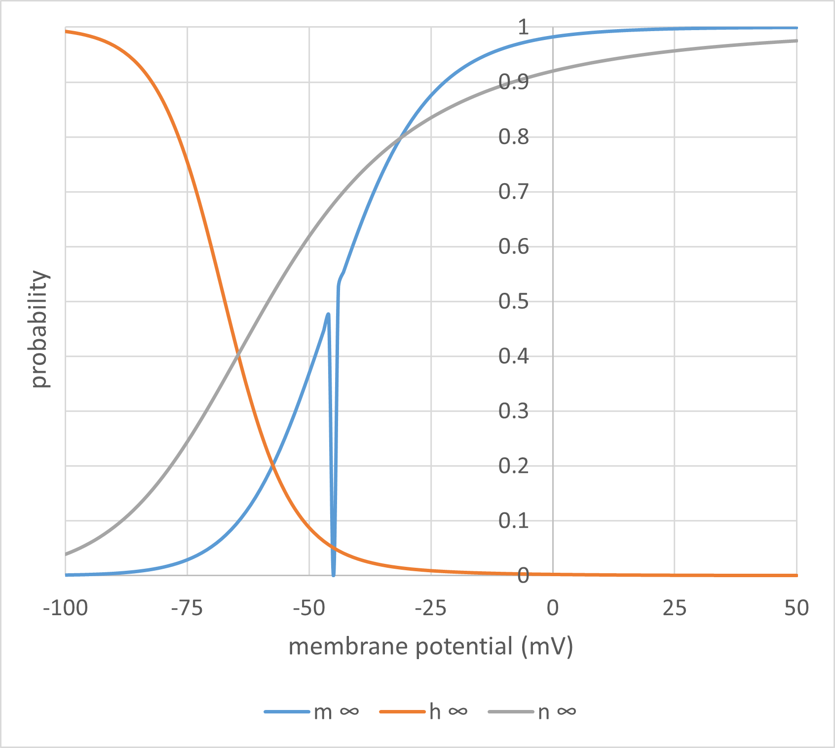
Clearly, if the membrane potential changes, and consequently the values of \(\boldsymbol{\alpha}\) and \(\boldsymbol{\beta}\) change, then the open probability P must also change. However, while \(\boldsymbol{\alpha}\) and \(\boldsymbol{\beta}\) change instantly with a change in voltage, this does not lead to an instant change in the value of P. This was discussed qualitatively above, but now we can quantify it. The rate at which P achieves its new value is equal to the difference between the rate of opening \eqref{eq:eqFracGatesOpening} and the rate of closing \eqref{eq:eqFracGatesClosing}:
\begin{equation} \frac{dP}{dt} =\alpha (1-P) - \beta P \label{eq:eqDerivAlphaBetaP} \end{equation}
Thus, following a change in voltage, the rate of change of P, as well as the direction and size of change, is dependent on the values of \(\boldsymbol{\alpha}\) and \(\boldsymbol{\beta}\) . Because different classes of gate are likely to have different values of \(\boldsymbol{\alpha}\) and \(\boldsymbol{\beta}\) at a given voltage, some classes of gates will respond more rapidly to changes in voltage than others.
Note:
The differential equation \eqref{eq:eqDerivAlphaBetaP} has an explicit solution in the form of a bounded exponential curve
\begin{equation} P_{t} = P_{\infty} - (P_{\infty}-P_{0})e^{-t/\tau} \label{eq:eqGateAlphaBetaP} \end{equation}
where \(\tau\) is the time constant and
\begin{equation} \tau = \frac{1}{\alpha + \beta} \label{eq:eqGateTimeConst} \end{equation}These equations can be understood as follows. We start with assuming that the system has been at a fixed constant voltage for a long period of time, and therefore P is at a starting equilibrium value P0 defined in equation \eqref{eq:eqGateInfinity}. The voltage then changes suddenly, and \(\boldsymbol{\alpha}\) and \(\boldsymbol{\beta}\) immediately switch to new values appropriate to the new voltage, according to equations \eqref{eq:eqAlphaBetaVoltDep}. P then starts to change, and approaches its new equilibrium value \(P_{\infty}\) (also defined in equation \eqref{eq:eqGateInfinity}, but with the new values for \(\boldsymbol{\alpha}\) and \(\boldsymbol{\beta}\) ) with an exponential time course with a time constant of \(\tau\). If either \(\boldsymbol{\alpha}\) or\(\boldsymbol{\beta}\) are large, then the time constant is short and P arrives at its new value rapidly. If both are small, then the time constant is long and it takes longer for P to reach equilibrium.

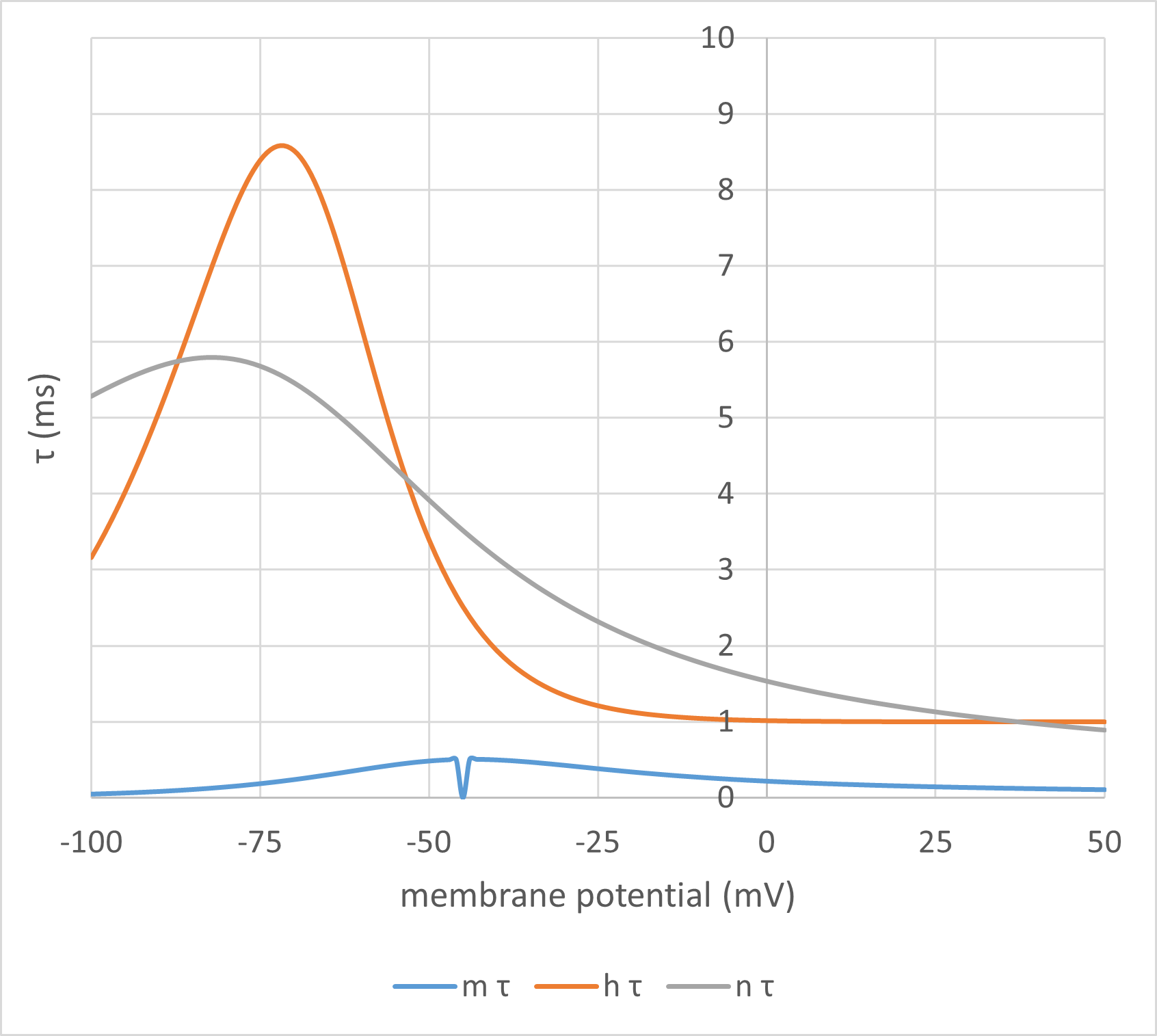
Fig. 5: Points of interest:
Here is an illustration of how these properties affect the response to a voltage shift.
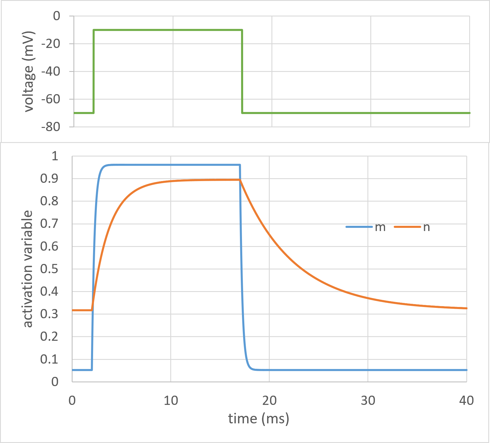
Fig. 6: Points of interest:
By combining equations \eqref{eq:eqGateInfinity} and \eqref{eq:eqGateTimeConst} it is possible to express \(\boldsymbol{\alpha}\) and \(\boldsymbol{\beta}\) in terms of \(P_{\infty}\) and \(\boldsymbol{\tau}\):
\begin{equation} \alpha = \frac{P_{\infty}}{\tau} \label{eq:eqAlphaAsPInf} \end{equation}
and
\begin{equation} \beta = \frac{1-P_{\infty}}{\tau} \label{eq:eqBetaAsPInf} \end{equation}
and the differential equation \eqref{eq:eqDerivAlphaBetaP} as:
\begin{equation} \frac{dP}{dt} = \frac{P_{\infty} - P}{\tau} \label{eq:eqDerivInfTauP} \end{equation}There is thus a simple relationship between \(\boldsymbol{\alpha}\) and \(\boldsymbol{\beta}\) , and the equilibrium value of P and the time constant \(\boldsymbol{\tau}\) with which P attains this equilibrium value.
Although the \(\boldsymbol{\alpha}\), \(\boldsymbol{\beta}\) values are foundational to the HH model, personally, I find the P\(\boldsymbol{\infty}\), \(\boldsymbol{\tau}\) formulation much easier to understand intuitively in terms of the consequences of their value. If you want to try out different values of these parameterst to see their interaction, the Excel tutorial worksheet alpha-beta provides a simple implementation of their formulaic relation.
Let us start the next stage of analysis by considering the situation when the voltage is stable, as it is when the membrane is sitting at the resting potential. For each class of gate in each type of channel, \(\boldsymbol{\alpha}\) and β have values appropriate for the voltage, and P (the probability of a gate being open) is at its steady-state equilibrium value given in equation \eqref{eq:eqGateInfinity}. If a channel contains several (say x) gates of that class within it, the probability of the whole channel being open is P raised to the power of the number of gates within the channel (i.e. Px). This is because all the gates have to be open for the channel to be open.
For reasons that will be explained later, HH proposed that each K channel has 4 identical activation gates (x = 4). We can replace the general probability value P with the specific probability of a K-channel n-gate being open, n, so the probability of a whole K channel being open is n4. Thus, to make this concrete, if at a particular voltage the probability of an n-gate being open is one half (n = 0.5), then the probability of an individual K channel being open is 0.5*0.5*0.5*0.5, or 1 in 16 (= 0.0625). By scaling up, we can say that 1 out of every 16 in the whole population of K channels will be open, and thus the actual K conductance (gK) will be 1/16th of the maximum possible K conductance, i.e.
\begin{equation} g_{{\small K}} = n^{4} g_{{\small K \, max}} \label{eq:eqN4} \end{equation}
where gK max is the membrane K conductance when all the K channels are open.
The HH model proposes that the Na channel has 3 activation m-gates, and one inactivation h-gate, and so by the same reasoning the Na conductance is
\begin{equation} g_{{\small Na}} = m^{3}h g_{{\small Na\, max}} \label{eq:eqM3H} \end{equation}
Once the conductance of a population of ion channels is known, the ionic current that flows through the channels can be calculated. This is because there is usually a fairly simple relationship between current (I), conductance (g), membrane potential (Vm) and the reversal (equilibrium) potential (Veq) of an ion, when the current is carried by that single ion species:
\begin{equation} I = g(V_m - V_{eq})\label{eq:eqCurrent} \end{equation}
This equation is a variant of Ohm's law. The factor Vm- Veq, which is a measure of how far the membrane potential is from the equilibrium potential of the ion in question, is called the driving force on the ion, and is equivalent to straight voltage in Ohm's law. We can make this equation specific for K ions
\begin{equation} I_K = g_K(V_m - V_{K\,eq})\label{eq:eqKCurrent} \end{equation}
where IK is the K current and VK eq is the K equilibrium potential. A similar equation gives the Na current
\begin{equation} I_{Na} = g_{Na}(V_m - V_{Na\, eq})\label{eq:eqNaCurrent} \end{equation}
There is a third current we have to consider: the leakage current. As well as the voltage-dependent channels discussed above, the membrane has a small, non-voltage-dependent conductance to both Na and K. This is known as the leakage conductance, and it is always present and remains constant whatever the voltage. The K component of the leakage conductance is much higher than the Na component (although both are small compared to the voltage-dependent conductances when they are activated), and so the leakage conductance acts as if it had an equilibrium potential close to resting potential.
\begin{equation} I_{leak} = g_{leak}(V_m - V_{leak\,eq})\label{eq:eqLeakCurrent} \end{equation}
It is intuitively obviousPossibly a very irritating phrase, since what may be obvious to the author may not be obvious to the reader. However, hopefully, in this case, it is. that if there is an imbalance in current across the membrane such that more positive charge enters the cell than leaves it, the accumulation of positive charge inside the cell will change the membrane potential and cause it to depolarise (make the inside more positive relative to the outside) and vice versa. More specifically, the change in membrane potential occurs because the unbalanced current alters the charge on the membrane capacitor. This is expressed by the following relationship:
\begin{equation} C_m\frac{dV}{dt} = I_{stim} - I_{ionic}\label{eq:eqCurrentBalance} \end{equation}
In this equation the expression Cm (dV/dt) is the capacity current (i.e. the rate at which charge builds up on the capacitor), and it derives simply from the property of capacitance, which says that the rate of change of voltage (dV/dt) across a capacitor is proportional to the current flowing into it, with the constant of proportionality being the value of the capacitor (effectively, its size). The equation states that the capacity current is equal to the arithmetic sum of all the other currents - this follows from the fact that if there is an imbalance between positive and negative "other" current, the “spare” current has nowhere else to go except into the membrane capacitor (but see note below). The "other" current consists of the ionic current Iionic , which is the sum of the Na, K and leakage currents calculated from the modified Ohm's law given above in equations \eqref{eq:eqKCurrent} - \eqref{eq:eqLeakCurrent}, plus any stimulating current Istim that is injected. If the sum of all these currents is 0, then no charge enters or leaves the capacitor, and there is no change in voltage across the membrane.
Note:
We can re-write equation \eqref{eq:eqCurrentBalance} thus
\begin{equation} \frac{dV}{dt} = \frac{I_{stim} - I_{ionic}}{C_m}\label{eq:eqDVbyDT} \end{equation}
In the resting neuron by definition the membrane potential is not changing, i.e. dV/dt (the rate of change of voltage) is 0. There is no stimulus applied, so Istim is 0, and therefore Iionic must also be 0. This does not mean that no ions are flowing through the channels across the membrane in the resting state, but it does mean that the inward and outward currents exactly balance to cancel each other, which, of course, is what you would expect for a resting neuron.
Now imagine what happens if a stimulus is applied to the neuron, so Istim is not 0. Initially Iionic does not change because none of the right hand sides of equations \eqref{eq:eqKCurrent} - \eqref{eq:eqLeakCurrent} changes, and therefore the stimulus current flows into the membrane capacitor and dV/dt becomes non-zero. Thus at the next instant in time, the membrane potential V has a new value. This has 2 effects. First, it will instantly change the driving force on all ions \eqref{eq:eqCurrent}. Second, it will instantly change the values of α and β for the channel gates, which will start to change the value of P for each of the gate classes \eqref{eq:eqDerivAlphaBetaP}. If P (i.e. m, n and h) changes, then the channel conductance g will change \eqref{eq:eqN4} and \eqref{eq:eqM3H}. A change in both conductance and driving force is very likely to result in a change in ionic current \eqref{eq:eqKCurrent} - \eqref{eq:eqLeakCurrent}, and this in turn is likely to lead to a further change in voltage \eqref{eq:eqDVbyDT}. In this way an iterative feedback process is initiated. The triumph of the HH model is that when you put all these equations together with the appropriate parameters, the voltage changes have the waveform of an action potential!
The original work of Hodgkin and Huxley (and some others) consisted of a three-stage process.
They proposed the basic model consisting of a membrane containing independent ion-specific channelsMembrane-spanning ion channels had not actually been discovered when HH proposed their model, and they called their ion-permeant entities "particles". , each of which contains voltage-dependent gates following first order kinetics. Currents through the channels are carried entirely by ions moving down electrochemical gradients. This is simple to state, but since there are very many alternative models that could have been proposed (such as ions transported across the membrane by lipid-soluble carrier molecules), this was a very insightful step. This theoretical framework led them to develop the equations described in the preceding sections of the tutorial.
In order to use the abstract equations they developed, they had to find appropriate numerical values to fill in the unknown parameters. There were 3 levels of detail required. First, the macro characteristics of the channel types (ionic specificity, maximum conductances, equilibrium potentials), had to be determined. Second, the number of activation and inactivation gates in each channel type had to be determined. Third, equations had to be found to describe the quantitative voltage dependency of α and β for each gate type in each voltage-dependent channel type.
The fact that Na and K are the major ions involved in generating the squid action potential had been established in earlier work, as had the equilibrium potentials for those ions. HH used ion substitutions to treat Na and K currents separatelyThe drugs TTX and TEA were not available in those days., and used the voltage clamp technique to measure the steady-state current at various voltages, and the rate of change of current following a change in voltage. Since the equilibrium potentials were known, the Na and K conductances could be determined from the current records using equations \eqref{eq:eqKCurrent} and \eqref{eq:eqNaCurrent}. This conductance data provide the necessary information to determine most of the remaining key parameters for the model. We will follow through the process for the K channels, because they are simpler than the Na channels since they do not inactivate.
In the HH model the K conductance changes with time after a step change in voltage according to this equation:
\begin{equation} g_t=\{g_\infty\,^{1/n} - [g_\infty\,^{1/n}-g_0\,^{1/n}]\,\textsf{exp}(-t/\tau)\}^n \label{eq:eqNGatesTime} \end{equation}
This equation is a modified version of equation \eqref{eq:eqGateAlphaBetaP}, where n is the number of gates in the channel. The equation applies (separately) to both the rising and falling phases of the clamp data, with g0 being the holding potential on the rising phase and the clamp potential on the falling phase, while g\(\boldsymbol{\infty}\) is the clamp potential on the rising phase and the holding potential on the falling phase. If the model is correct, n will have the same value for both the rising and falling phases and for any holding or clamp potential, since it is determined by the molecular structure of the channel, but the conductances and \(\boldsymbol{\tau}\) will vary according to the voltages used.
Here is a typical voltage clamp recording of the K current, including the calculated K conductance. This figure is actually generated by the model itself (so obviously cannot be used to verify the model), but comparison of the model conductance trace with that calculated from real experimental data (e.g. Fig. 2 in the key HH paper) confirms their similarity.
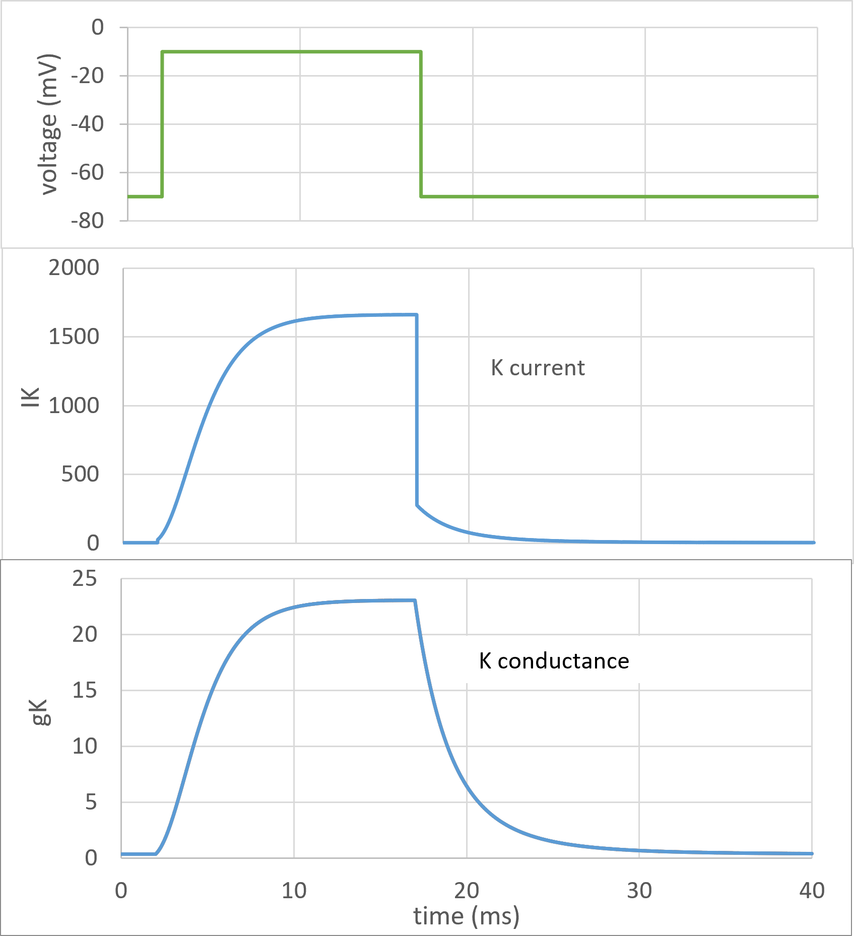
Fig. 7: Points of interest:
Fig. 7 shows that during the depolarising step of a voltage clamp experiment the K conductance change has an asymmetric sigmoid shape, but during the repolarising step the conductance change has an exponential shape (shown with real data in Fig. 2 in the key HH paper). HH knew that single first-order reactions of the type proposed for the individual channel gates should produce exponential curves, but that sigmoid curves would result from co-operative processes in which several first order reactions had to occur simultaneously. This fitted with the notion that the channels contained several gates, all of which had to be open at once in order for the channel itself to be open, hence the sigmoid shape of the rising curve. On the other hand, only one gate had to shut for the channel to shut, hence the exponential shape of the falling curve. In co-operative processes, the shape of the sigmoid part of the curve depends on the number of events involved; the greater the number of events, the more pronounced the inflexion on the rising phase of the curve.
The difference in shape can be visualized by running a modified HH model with different numbers of gates in the K channel.
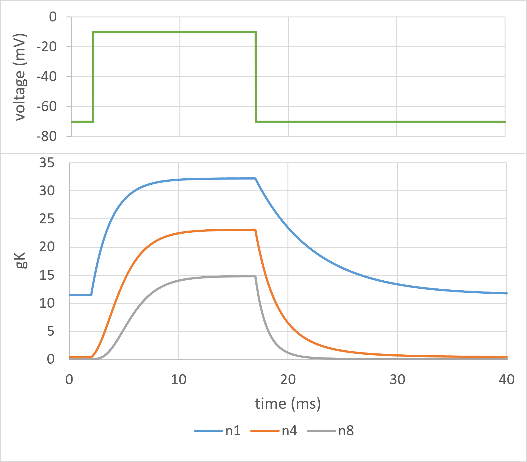
Fig. 8: Points of interest:
HH found that the n4 profile provided the best fit to the experimental data for both rising and falling phases, so 4 could be substituted for n in equation \eqref{eq:eqNGatesTime}. Then, by curve fitting the rising phase of the conductance to the equation, the time constant \(\boldsymbol{\tau}\) can be found at the clamp potential (-10 mV in Fig. 8), and by curve fitting the falling phase, the time constant at the holding potential (-70 mV) could be established. Note that the time constant found by curve-fitting to the equation is the time constant of the gate state change, not the time constant of the conductance change visible in the clamp data.
Analysis of the Na conductance was more complicated due to the inactivation process (indeed, an entire paper was devoted to this topic alone), but in essence the process was the same - finding the combination of activation and inactivation gates that provided the best fit to the data.
By performing voltage clamp experiments using a range of clamp potentials, HH could establish the steady-state K conductance at each potential as a fraction of the maximum possible K conductance, and the 4th root of this (rearranging equation \eqref{eq:eqN4}) gave a value for the steady-state n-gate open probability n\(\boldsymbol{\infty}\) at that voltage. The curve fitting described above gave values of the time constant n\(\boldsymbol{\tau}\) at each voltage.
We have seen earlier (equations \eqref{eq:eqAlphaAsPInf} and \eqref{eq:eqBetaAsPInf}) that for any gate type there is a simple relation between the values of the transition rate constants \(\boldsymbol{\alpha}\) and \(\boldsymbol{\beta}\), the fraction of gates in the open state P (n\(\boldsymbol{\infty}\) for K channels), and the time constant with which that fraction approaches its steady-state value τ (n\(\boldsymbol{\tau}\) for K channels). This means that if P and \(\boldsymbol{\tau}\) are known for particular voltage, then \(\boldsymbol{\alpha}\) and \(\boldsymbol{\beta}\) can easily be calculated.
So now HH had values for \(\boldsymbol{\alpha}\) and \(\boldsymbol{\beta}\) for the n gate of the K channel over a range of voltages. The values showed smooth continuous changes over the physiological voltage range, so all (!) they had to do was find a set of mathematical functions that described those changes. The functions they came up with are those given in Table 1 above \eqref{eq:eqAlphaBetaVoltDep}.
Having derived the model and its equations as described above, and having determined the appropriate numerical parameters by experiment, HH then worked forwards and "reconstructed" the effects of applying a depolarising stimulus to an axon. This was done by numerical integration of the equations.
Solving the HH equation (i.e. calculating the value of the membrane potential as time passes) requires solving 4 differential equations simultaneously. Three equations (\eqref{eq:eqGrandHH1} - \eqref{eq:eqGrandHH3}) are like equations \eqref{eq:eqDerivAlphaBetaP} or \eqref{eq:eqDerivInfTauP} and use the instantaneously voltage-dependent factors to describe the rate of change in the gating variables:
\begin{align}
\frac{dm}{dt} &= \alpha_{m(V)}(1-m)-\beta_{m(V)} &&= \frac{m_{\infty(V)} - m}{\tau_{m(V)}} \label{eq:eqGrandHH1} \\[1.5ex]
\frac{dh}{dt} &= \alpha_{h(V)}(1-h)-\beta_{h(V)} &&= \frac{h_{\infty(V)} - h}{\tau_{h(V)}} \label{eq:eqGrandHH2} \\[1.5ex]
\frac{dn}{dt} &= \alpha_{n(V)}(1-n)-\beta_{n(V)} &&= \frac{n_{\infty(V)} - n}{\tau_{n(V)}} \label{eq:eqGrandHH3}
\end{align}
Integrating these equations yields the moment-by-moment values for m, h and n in the HH model. Once these values have been calculated, they are put into equations \eqref{eq:eqN4} and \eqref{eq:eqM3H} to calculate the potassium and sodium channel conductances. Once the conductances are known, the driving force equation \eqref{eq:eqCurrent} is used to calculate the current flowing through each ion channel type (sodium, potassium and the fixed-conductance leakage channels). So the end point of this is that we know the currents through the ion channels, and we know the stimulus current because we control that.
The fourth equation \eqref{eq:eqGrandHH4} depends on Kirchoff’s rule, which states that the sum of currents entering and leaving any point in a circuit is zero. Since the only pathsAssuming the cell is isopotential and that there is no internal current flow to a different region such as an axon or dendrites. If there is such lateral flow, you need to build a compartmental model. into or out of the cell are through the membrane capacitance or the membrane conductance, their currents must be equal and opposite in order to achieve a total of zero. The current charging a capacitor is directly proportional to the rate of change of voltage over the capacitor, as given by equation $I = C\,dV/dt$, so the rate of change of voltage multiplied by the constant of proportionality (the capacitance) must be equal to the total current through the ion channels, plus any stimulus current. This leads directly to the fourth equation:
\begin{equation} \begin{aligned} C\frac{dV}{dt} = I_{stim} &- g_{Na\,max}m^{3}h(V-E_{Na}) \\ &-g_{K\,max}n^{4} (V-E_{K}) \\[1.5ex] &-g_{leak}(V-E_{leak}) \end{aligned} \label{eq:eqGrandHH4} \end{equation}Integrating this equation is what actually calculates the membrane potential V at each moment in time.