a
b

c

We will start by producing a model of the passive membrane, i.e. an RC circuit where the R component only contains the leakage channels. This is simpler than the full HH model because it only requires integrating one differential equation - a modified version of equation (25). The other 3 equations which need integrating in the full model are concerned with the m, h and n gates of the voltage-dependent channels, which are not included in this initial model.
The relevant equation is
\begin{equation} \frac{dV}{dt} = \frac{I_{stim} - g_{leak}(V - E_{leak})}{C_m}\label{eq:eqPassiveMembrane} \end{equation}
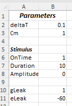
The model is available in the Passive membrane worksheet in the tutorial Excel file. If possible, open that file and display it alongside this browser window.
The key spreadsheet formulae for integrating the equation using the Euler method are shown below:
Integrating equation \eqref{eq:eqPassiveMembrane} for 20 ms using the default parameters in the supplied Excel model yields this voltage profile:
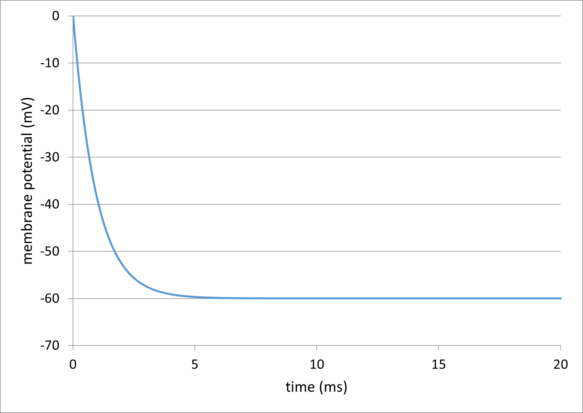
The reason for the fall on the left hand side in Fig. 13 is that the initial value for the membrane potential is 0, but the steady state (dV/dt = 0) value in \eqref{eq:eqPassiveMembrane} is when V = Eleak, and Eleak has been set to -60 (cell B10 in the spreadsheet).
In the Excel file, set the initial membrane potential (cell E2) to -60. The Excel plot should immediately switch to a flat line at -60, which is the leakage channel equilibrium potential. Since this is the only channel type in the membrane, this sets the resting potential.
Now set the stimulus amplitude (cell B8) to 1. This should generate this voltage profile:
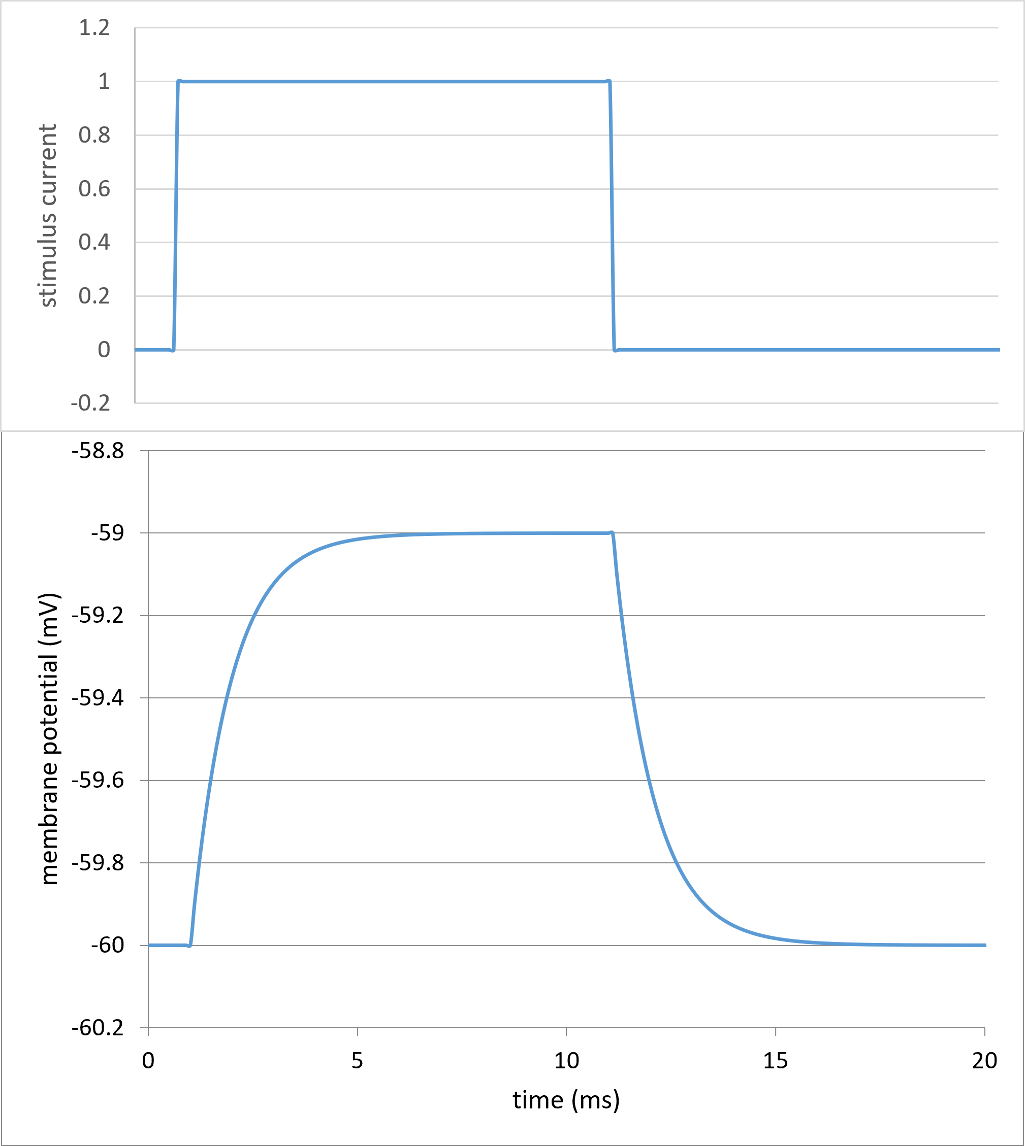
This is the classic RC response to a brief stimulus current. The peak (stable) voltage deflection allows the input resistance to be measured using Ohm's law. The rising and falling curves both follow a bounded exponential waveform with a time constant equal to the product of membrane capacitance and resistance (this is the physics rule for an RC circuit). If you adjust the leak conductance(B10; conductance is just the reciprocal of resistance) and membrane capacitance (B3) values, you can see how these paramaters effect the membrane response to the current stimulus.
The ultimate aim of this section of the tutorial is to produce an Excel version of the HH model that, with an appropriate stimulus, generates an action potential. We can pick up lots of other information about other parameters along the way, but that is the key purpose.
The full HH model is available in the HH worksheet in the tutorial Excel file. If possible, open that file and display it alongside this browser window. The worksheet is quite complicated, so we will deal with it in sections.
At the top-left area of the spreadsheet there is a set of single value named cells in column B that contain user-editable content:
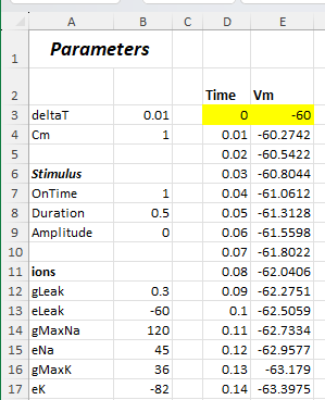
Other than the single-value named cells in column B, only two values in the integration process are explicitly specified, the initial time and voltage (the yellow highlighted cells in Fig. 15). These are the specified x, y pair required to integrate ODEs consituting an initial value problem. The initial time (Time: D3) is set to 0 and will not be changed. The initial voltage (Vm: E3) is set to the same value as the leakage equilibrium potential (-60), but this will be adjusted later.
Some of the formulae in the first row are different from subsequent rows, because it is assumed that the system is in steady-state at time 0. It is as if a voltage clamp of the initial membrane potential had been applied before time 0, but this notional clamp is released after time 0.
The first task at each step of the integration is to find the transition rate constants \(\boldsymbol{\alpha}\) and \(\boldsymbol{\beta}\) for the 3 gate types (m, h and n), since these are foundational to all the voltage-dependent channel properties. This is done in columns V-AA. The values are only dependent on the voltage at that step, and at the start (row 3) we know the voltage is -60 because it is set as an initial value.
The worksheet makes extensive use of named ranges which start with the @ symbol, which means that the reference is to a value in the same row as the occurrence of the symbol. Thus cell V3 contains the formula for calculating the transition rate constant for \(\boldsymbol{\alpha}\)m (an Excel implementation of the equivalent HH equation) for row 3:
=(-0.1*(@Vm+45))/(EXP((@Vm+45)/-10)-1)However, the cells in all the data rows in that column contain exactly the same formula text. This works because the reference @Vm in cell V3 refers to the voltage value in cell E3, but the same reference in cell V4 refers to the voltage value in cell E4 etc.
In the first row alone, the transition rate constants allow immediate calculation of the activation variables m, h and n (green highlight) through equation (6) because it is assumed that the system is in steady-state at time 0. However, this equation does not apply to subsequent rows (see below) because the system is no longer in steady state.
We now have initial values of m, \(\boldsymbol{\alpha}\)m and \(\boldsymbol{\beta}\)m, so we can calculate the rate of change of m (dm/dt) in this state from equation (7). The same applies to the h and n gates. At this first row, all the rates of change are 0 because the m, h and n values have been calculated from equation (6), which assumes that the system is in equilibrium and so produces a zero rate of change. This will change in subsequent rows as the integration advances step by step.
We now know the values of the activation variables m, h and n at this time step. This gives us the conductance of the Na and K channels (gNa, gK: columns O, P) through equations (13, 14), which in turn give the Na and K currents (iNa, iK: columns L, M) from equations (16, 17). The leakage current (iLeak: column K) is calculated as for the Passive Membrane, as is the stimulus current.
Now we can calculate the rate of change of voltage (dV/dt: column H) using a version of equation \eqref{eq:eqPassiveMembrane} expanded to include the voltage-dependent channels:
=(@Stim-@iLeak-@iNa-@iK)/Cm
For the second row onwards, the Vm and m, h and n formulae (columns E, R-T) advance their value from that in the previous row by adding a step \(\Delta\) calculated by multiplying the appropriate derivative (columns H, AC, AD, AE) in the previous row by the time step deltaT (cell B3). E.g the formula for Vm in the second row (E4):
=E3+H3*deltaT
refers to its value in the previous row (E3) plus its derivative in the previous row (H3) muliplied by the user-determined single value time step deltaT. The same method is used to advance the gate variables m, h and n. (The named range @ symbol cannot be used here because the reference is to values in a different row to the formula.)
The graph showing a plot of voltage against time shows that the initial Vm is not a stable resting potential. Numerically, this is obvious because dV/dt in the top row is not even close to 0, and this in turn is because the sum of ionic currents (iTotal = ILeak + INa + IK) in the top row is not zero either, so from the outset there is an imbalance between the inflow and outflow of charge which will lead to a voltage change.
However, the graph also shows that the voltage stabilizes over time. The stable Vm can be read from its value later in the integration at the bottom row of the worksheet (cell E2296) where Vm = -70.2324 (and dV/dt is close to zero, as is the sum of the ionic currents).
In the Excel file, set the initial membrane potential Vm ( cell E3) to -70.2324. The graph now changes to a flat line, so this is a stable resting potential that we can use from now on.
Set the singe value stimulus Amplitude (cell B9) to 10. There is a deflection in the Vm trace that considerably outlasts the stimulus, indicating that voltage-dependent channels have been affected by the stimulus, but there is no spike. The stimulus is subthreshold.
Increase the Amplitude to 15. The Vm trace now shows a spike. SUCCESS!!!
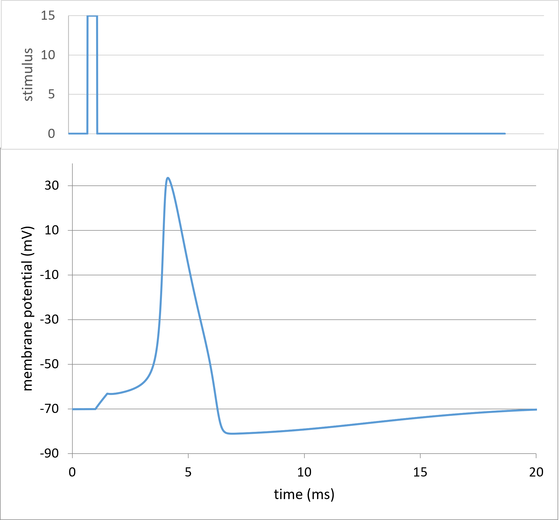
If you wanted to dig deeper into the mechanism of the spike, you could plot any of the underlying variables such as the Na or K currents, conductances etc. However, the main purpose of this tutorial is to explain the model rather than to explain the spike, so I will leave that up to the reader.
Earlier in the tutorial on Integration methods, it was emphasised that Euler integration only yields reasonable results if the step size \(\Delta\) is kept relatively short. How short is short enough?
Halve the step size deltaT (cell B3) by entering 0.005. There is a very slight shift in the spike timing, but the waveform is virtually identical (it is truncated because we would need to extend the spreadsheet columns to fill data up to 20 ms). This suggests that the original value of 0.01 was satisfactoryThat sort of shift would not be acceptable if you were flying a rocket to Mars, but in the HH model all the parameter values are estimated from experimental results containing noise, and small changes in their values can also produce similar changes in the results, so obsessive concentration on integration accuracy is not really necessary for our purposes. If you needed greater accuracy, you would use a more sophisticated integration algorithm than the forward Euler method..
Now set deltaT to 0.1 (10x longer than the original step size). The initial part of the waveform looks OK, but at about the peak of the action potential, the integration "blows up". There are a few wild oscillations, followed by a flat line at 0 caused by not-a-number results due to divide-by-zero errors.
In some ways, catastrophic failure like this is better than results that might be right, but are in fact wrong. Try a deltaT value of 0.07. This produces a spike waveform that is correct in its overall appearance, but has spurious oscillations on the falling phase. If we didn't know better, we might think that these were a genuine biological phenomenon, whereas they are in fact an artefact caused by too large an integration step size.
The take-home message is that it is usually a good idea to check whether a reduction in step size produces a significant change in output, and if it does, to keep reducing the step size until it doesn't. However, you should also be aware that too small a step size can also cause an increase in accumulated error because of the greater number of steps involved.
HH found that their model successfully reproduced several secondary spike-related phenomena, such as the refractory period and post-inhibitory (anode break) excitation. To demonstrate the refractory period would require modifying the Excel implementation to include a second stimulus, which would be quite easy, but which I will leave to the reader.
Rebound excitation can be demonstrated simply by making the stimulus negative.
Return the deltaT step size to 0.01, and then set the stimulus Amplitude to -40. The membrane undergoes a brief hyperpolarization during the negative stimulus, and then generates a spike on rebound from that stimulus. By looking at the underlying variables, the explanation for the rebound offered by HH can be verified - the hyperpolarization reduces the K conductance and removes Na inactivation, and these effects are relatively long lasting due to the long time constants of the relevant gates within this range of the membrane potential.
A slight modification of the Excel code transforms it from the HH current clamp model into a voltage clamp model. In a voltage clamp experiment the membrane potential is set by the user, so this model only requires integrating 3 differential equations; those controlling the m, h and n activation variables (equations 22-24). The Excel implementation is available in the Voltage Clamp worksheet in the tutorial file. If possible, open that file and display it alongside this browser window.
As before, the cells in column B at the top left of the worksheet contain single values set by the user.
Some of the logic of the integration code is the same as for the current clamp model. In each integration step (row) the first task is to find the transition rate constants \(\boldsymbol{\alpha}\) and \(\boldsymbol{\beta}\) for the 3 gate types. This is done in columns S-X. The values are dependent on the voltage Vm at that step, which initially is the holding potential (HoldPot = -70). However, unlike in the current clamp model, in the voltage clamp we know the Vm value throughout the whole simulation because it is set by the user, and is either the holding potential (HoldPot) or the clamp potential (ClampPot).
As before, in the first row the rate constants directly sets the activation variables m, h and n values from their steady-state equation (6). These in turn set the conductances and hence currents for the leakage, Na and K channels. The rate constants also set the rate of change (derivative) of the activation variables from equation (7). Initially the derivative is 0 because the system has been in steady-state before time 0. However, unlike in the current clamp model, the derivative remains at 0 until the clamp potential (Vm) changes at the clamp on time (OnT: cell B8) set by the user. Because their derivative is 0 until the clamp potential changes, the activation variables themselves do not change until the potential changes. So everything remains in the initial state until the voltage clamp switches to a new voltage value.
Once the voltage switches to the clamp potential (ClampPot = -10, OnT = 0.5 at row 53) there is a new set of values for the transition rate constants but, initially, the previous value of the gate activation variables. Since the derivative of the activation variables depends on both their rate constants and their instantaneous values (equation 7), and their instantaneous values are still at those of the holding potential in the previous step, there are now new , non-0 derivatives for the activation variables. So at the next integrations step, m, h and n start to change towards a new steady state value appropriate for the new clamp potential. And as the activation variables change, so do the conductances and currents. If the new clamp potential is maintained long enough, eventually m, h and n attain their steady-state values at that potential, and once again the system is stable with nothing changing until Vm changes on return to the original holding potential.
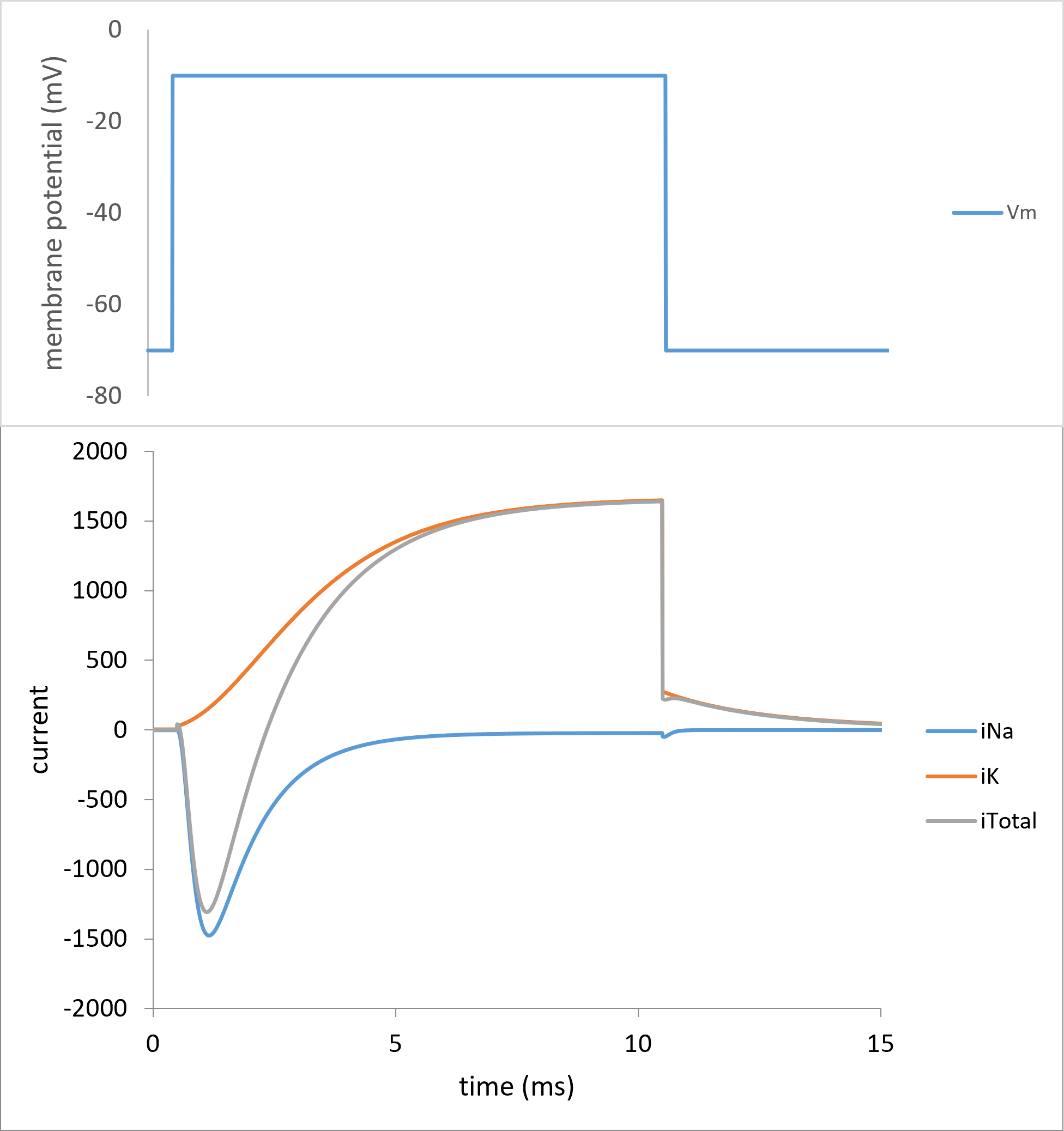
Figure 17. Voltage clamp from the HH model. The clamp is stepped from -70 to -10 mV and back (top trace). The Na, K and total currents are displayed (bottom traces).
THAT'S IT, FOLKS!
Hopefully, you now have some understanding of the HH model of the action potential, and also some knowledge about how it can be implemented in Excel.
I hope you found this useful (and perhaps even enjoyable!).