The easiest way to load a parameter file is by drag-and-drop from File Explorer, although you can certainly use the File: Open menu command, or the button on the main toolbar if you wish.
If you double-click a parameter file in File Explorer it will activate a new instance of Neurosim with the file pre-loaded.
Web Links
If you click on a web-link to a parameter file, you may be asked whether you want to download or run it. If you select run, be aware that a local copy of the file may be downloaded to your default Download folder, depending on your browser. To prevent disk clutter, you may want to delete these files after you finish your simulation session.
Each link activates a new instance of Neurosim, similar to double-clicking a local file.
In this Neurosim tutorial, parameter file links are shown in green thus.
Check the Measure box at the top of the Results view to open the Measure dialog.
If necessary, move thedialog so that it does not obscure the Results view.
The dialog is non-modal, so can be kept open while you do experiments
Drag the red cursor in the Results view to the X-location at which you want to make the measurement.
You can fine-position the cursor with the < and > buttons.
Click the Measure button in the Measure dialog. Note that the data value of each trace appears in the dialog in the labelled columns.
If there is more than one sweep, data are measured from each sweep in sequence unless a sweep is highlighted in the Results view, in which case only data from that sweep are measured.
Repeat the measurements at different X-locations as necessary.
Dual Cursors
You can measure values and their differences at two different times using dual cursors.
Check the 2 cursors box.
A blue cursor now appears in addition to the red cursor.
If you only want the difference between cursor values, check the Only difference box.
You can change which cursor is moved by the < and > buttons by selecting Red or Blue from the radio button choice.
User column
You can add a column to enter a user-specified value or label to each measurement row if desired:
Click the +User button to add a column at the left of the measurements.
Click the column header to edit its label if desired.
Click each cell in the user column and enter appropriate data.
You can navigate between rows with up- and down-arrow keys.
Plot
Click the Plot button to activate an X-Y scatter plot of the measurements.
Select which parameter goes on which axis from the axis drop-down list.
Context-sensitive help is available at any time within Neurosim by pressing F1.
Add horizontal and/or vertical cursors to the display by:
clicking the appropriate Results toolbar button ( or ), or
selecting from the View: Cursors menu, or
right-clicking in the Results view and selecting from the context menu.
Position cursors by dragging with the mouse.
You can adjust the fine position of a selected cursor using the keyboard arrow keys. A cursor is selected by clicking it. A selected cursor is indicated by the blue bar at its end.
The time (vertical cursor) or trace value (horizontal cursor) at the cursor location shows at its top or left end. The value labels can be dragged along the cursor to a more convenient screen location if desired. IMPORTANT: for horizontal cursors, the value is that for the axis range in which the cursor is located.
If you have multiple cursors displayed they can be coupled together so that when you move one cursors, all cursors of the same type move by the same amount. This option is available on the View: Cursors menu.
Cursors can be deleted by right-clicking within the Results view, and selecting the appropriate command from the context menu.
The transmembrane current carried by ions flowing through an ion channel is given by the following equation:
I = g(Vm-Veq)
where I is the current, g is the conductance of the channel to the ion, Vm is the membrane potential, and Veq is the equilibrium potential of the ion in question.
The factor (Vm - V eq) is known as the driving force, because the further the membrane potential is from the equilibrium potential of an ion, the greater the “push” on the ion resulting from the imbalance in the Nernst equation.
This equation is a simple variant of Ohm's Law (current = conductance x voltage), but voltage is represented by the driving force. It is one of the most important equations in cellular electrophysiology because it allows us to quantifiy current flow in both action potentials and chemical synapses.
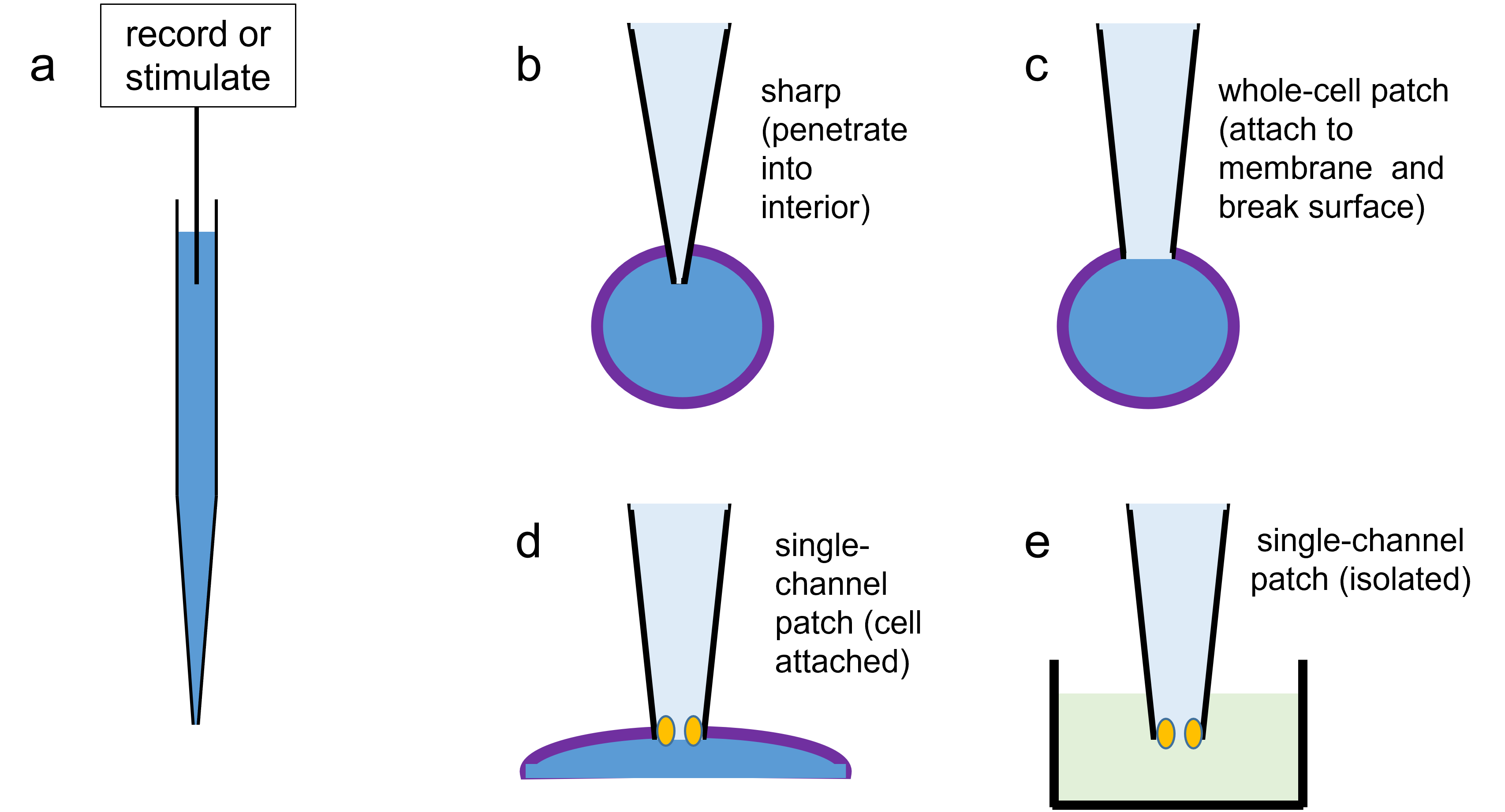
Four different recording methods. a. Intracellular recording usually involves a microelectrode - a glass tube drawn out to a very fine point and filled with an electrolyte. The blunt end of the tube is connected by a wire to a recording amplifier or stimulator. b. A sharp microelectrode penetrates into the interior of the cell. This can record the membrane potential or inject current. c. A patch electrode attaches to the cell surface and breaks the membrane just under its tip. This can record and stimulate like method a, but usually causes less damage to the cell. Also a patch electrode is usually blunter than a sharp electrode, and passes current more easily and records with less noise. d. A patch electrode attaches to the cell surface with just a single ion channel under its tip. This can record the current through that channel, with the rest of the cell still attached and undamaged. e. As d, but the electrode is withdrawn from the cell, bringing the single channel with it. Current flowing through the channels can be recorded, and the chemical environment on both sides of the channel can be controlled by the experimenter. By careful manipulation the channel can be arranged to have its inner surface within the electrode lumen (outside-out patch) or its outer surface within the lumen (inside-out patch).
Many transfer functions of the form y = f(x) allow the user to choose between linear, sigmoid, and user-specified types. In each case there may be a specified minimum and maximum output.
Linear: There is linear interpolation between the minimum and maximum. Two parameters control the function:
Threshold: Below this input level, the output is the minimum.
Saturate: Above this input level, the output is the maximum.
For input between the threshold and saturate levels, the output scales linearly:
\begin{equation}
y = min + (max - min) \times (x - thresh) / (sat - thresh)
\label{eq:eqLinearTrF}
\end{equation}
Sigmoid: The function has a sigmoid shape varying between the minimum and maximum. Two parameters control the shape of the sigmoid:
Mid: The input value that produces output mid way up the curve of the sigmoid shape.
Slope: The steepness of the sigmoid curve. Often the inverse slope is used, so larger values produce shallower slopes.
\begin{equation}
y = min + (max - min)/(1+e^{\frac{mid-x}{slope}})
\label{eq:eqSigmoidTrF}
\end{equation}
User: The user specifies an equation using the built-in expression parser. Context-dependent parameters may be passed to the equation. It is up to the user to ensure that the output is appropriate for the intended use.
Select 0 (new) in the Experimental Contol panel.
The panel is normally docked on the left of the Setup view, but it can be floated, or docked elsewhere if desired.
Edit the stimulus parameters as desired.
Enter the appropriate ID number(s) into the Target neuron(s) box. You can apply the same stimulus to multiple neurons by entering multiple numbers.
Select an Existing Stimulus
Either Click on the appropriate square box attached to the target neuron in the Setup view
Or
Click on the stimulus number in the Stimulus list in the Experimental Control panel.
Edit an Existing Stimulus
Select the stimulus as above.
Edit the parameters in the Stimulus list in the Experimental Control panel.
Change the Target of an Existing Stimulus
Either Drag the square stimulus box from the existing target neuron to the new target neuron in the Setup view.
Or
Select the stimulus number in the Stimulus list in the Experimental Control panel.
This section describes in detail the kinetic equations that underlie the Hodgkin-Huxley model, and some of the advanced techniques used to analyse them. It can be safely IGNORED if this is beyond what is needed by the user.
The factors \(\alpha\) and \(\beta\) are the transition rate constants. \(\alpha\) is the number of times per second that a gate which is in the shut state opens, while \(\beta\) is the number of times per second that a gate which is in the open state shuts.
The key factor in the HH model which allows action potentials to be generated is that \(\alpha\) and \(\beta\) are voltage dependent. The equations defining the voltage-dependency for \(\alpha\) and \(\beta\) for the m, h and n gates are given in the table below.
\[{\large \beta_{n}} = 0.125 e ^ {\Large {\frac{V_{m}+70}{-80}}} \]
As can be seen, the only variable on the right-hand side of each equation is the membrane potential Vm. This means that \(\alpha\) and \(\beta\) are directly and instantaneously dependent on the membrane potential.
It is worth making three points about the equations:
The form of these equations, which are variants of the Boltzmann sigmoid function, is not arbitrary but is derived from physical chemistry theory.
The numerical constants are empirical estimates ultimately derived by curve-fitting of voltage clamp experimental data.
The value of the constants shown in this table have been adjusted from their original published values in order to use a normal voltage convention with a resting potential of -70 mV. HH had the resting potential as zero, and depolarization as a negative change in Vm.
So how does the open probability of a gate depend upon \(\alpha\) and \(\beta\)? For a whole population of gates, a proportion P are in the open state, where P varies between 0 and 1. This means that a proportion 1 - P will be in the closed state. The fraction of the total population which open in a given time is dependent on the proportion of gates which are shut, and the rate at which shut gates open:
\begin{equation}
\textsf{fraction of gates opening} =\alpha (1-P)
\label{eq:eqFracGatesOpening}
\end{equation}
and similarly
\begin{equation}
\textsf{fraction of gates closing} =\beta P
\label{eq:eqFracGatesClosing}
\end{equation}
From this we can construct a differential equation. The rate of change of P will be the difference between the fraction opening per unit time and the fraction closing:
\begin{equation}
\frac{dP}{dt} =\alpha (1-P) - \beta P
\label{eq:eqDerivAlphaBetaP}
\end{equation}
If \(\alpha\) and \(\beta\) are fixed, which they are if the voltage is stable, then this equation will naturally tend towards equilibrium (no change in P; dP/dt = 0). This is because if dP/dt is positive, then the rate of opening exceeds the rate of closing and P increases, which increases the rate of closing (βP) and decreases the rate of opening (α(1-P) so dP/dt becomes less positive. The same argument (in reverse) applies if dP/dt starts negative. So dP/dt ends up at zero.
When the system reaches equilibrium, the fraction of gates opening must equal the fraction of gates closing in any given period of time:
\begin{equation*}
\alpha (1-P) = \beta P
\end{equation*}
This means that if \(\alpha\) is high and \(\beta\) is low, the gate has a high probability of being open, and vice versa. (The infinity subscript is used for P because the system only achieves equilibrium if \(\alpha\) and \(\beta\) remain stable for a relatively long period of time.)
If the membrane potential changes, and consequently the values of \(\alpha\) and \(\beta\) change, then the open probability P will also change. However, this does not occur instantly, even though the \(\alpha\) and \(\beta\) changes are instant. The rate at which P achieves its new value from a starting value of P0 is equal to the difference in the rate of shutting and the rate of opening given in the differential equation \eqref{eq:eqDerivAlphaBetaP}. This has the explicit solution in the form of a bounded exponential curve:
Thus, following a change in voltage, the rate of change of P, as well as the direction and size of change, is dependent on the values of \(\alpha\) and \(\beta\). Depending on these values, some classes of gates will respond more rapidly to changes in voltage than others.
These equations can be understood as follows. We start with assuming that the system has been at a fixed constant voltage for a long period of time, and therefore P is at a starting equilibrium value \(P_{\infty}\) defined in equation \eqref{eq:eqGateInfinity}. The voltage is then changed suddenly, and \(\alpha\) and \(\beta\) immediately switch to new values appropriate to the new voltage, as defined by the equations in the table above. P then starts to change, and approaches its new equilibrium value \(P_{\infty}\) (also defined in equation \eqref{eq:eqGateInfinity}, but with the new values for \(\alpha\) and \(\beta\)) with an exponential time course with a time constant of \(\tau\) from equation \eqref{eq:eqGateTimeConst}. If either \(\alpha\) or \(\beta\) are large, then the time constant is short and P arrives at its new value rapidly. If both are small, then the time constant is long and it takes longer for P to reach equilibrium.
By combining equations \eqref{eq:eqGateInfinity} and \eqref{eq:eqGateTimeConst} we can express \(\alpha\) and \(\beta\) in terms of \(P_{\infty}\) and \(\tau\) :
There is thus a simple relationship between \(\alpha\) and \(\beta\), and the equilibrium value of P and the time constant \(\tau\) with which P attains this equilibrium value.
In the equations above, P is the open-probability of an unspecified gate type. However, in the HH model, we have the specific m, h and n gates. The same equations apply, just substitute the appropriate letter identifier for P.
Take-home message: To specify the voltage-dependent characteristics of a gate type, we can
either specify equations defining the voltage-dependency of \(\alpha\) and \(\beta\) as in the table above,
or specify a different but related set of equations defining the voltage-dependency of \(P_{\infty}\) and \(\tau\).
The Results display shows a voltage-clamp experiment, with the clamp potential in the top trace. However, the second trace is not current (as it would be in a real experiment), but rather the values of the open probabilityof thesodiumand potassium activation gates (m, orange trace, and n, blue trace, respectively). The sodium inactivation gate (h) is not shown to avoid confusion with too many lines crossing over. [Remember, these probabilities could never be measured directly in a real experiment - they are just part of the model, but in terms of understanding how the model works it is useful to display their values.]
Each time there is a step change in the voltage, the m and n values change to new steady-state values. However, the change is not instant, but rather occurs with what looks like an exponential time course.
This is particularly obvious for the n gate curve (blue trace) in the first clamp step.
So far so good - the model matches the theory given above.
Steady-State Probability
Click the Kinetics button in the Membrane Properties group in the Setup view.
The HH Kinetics dialog box opens with the Probability (\(t_{\infty}\)) display option selected.
The graph shows the steady-state (time infinity) values of m, h and n across a range of physiological membrane potentials. The sodium and potassium activation gates (m, orange and n, blue respectively) both increase their open probability with depolarization, and the sodium inactivation gate (green) decreases its open probability with depolarization, as they should.
Take-home message: m, h and n gates have steady-state open probabilities whose voltage-dependency reflects their roles in sodium channel activation, sodium channel inactivation and potassium channel activation respectively.
Question: The graph shows that the n line (blue potassium activation gate) is above the m line (orange sodium activation gate) at voltages below about -30 mV, but below it at more depolarized voltages. Does this qualitatively match-up with the steady-state m and n values shown in the Results view? The clamp potentials are -70, -60 and -10 mV.
Time Constant of Probability Change
Select the Time constant t display option in the HH Kinetics dialog.
Note that m (orange line) is low down on the graph and thus has a short time constant
at all membrane potentials (less than 0.5 ms).
In contrast, both h and n have relatively long time constants (6 - 8 ms) around the resting potential (left-hand part of the graph),
but this decreases significantly with depolarization (right-hand part of the graph).
Compare the m and n responses in the Results view. m (the orange trace) changes to its new value almost instantlyIn some published HH-type models m is assumed to have a fixed 0 or very short time constant, which can speed up computation by avoiding calculating the kinetic equations for m, without sacrificing too much accuracy., and this is true for both the rising and falling phases of the small depolarization (the first step) and the large depolarization (the second step). In contrast, n (the blue trace) responds quite slowly to both rising and falling phases of the small depolarization. This is because the membrane potential remains within the range in which the time constant is long. But it responds much more quickly to the rising phase of the large depolarization because the membrane potential has stepped into the region where its time constant is short. However, when the membrane potential steps back down to rest (the falling phase of the large step), the rate of change in n is again slow (much slower than it was on the rising phase), because the membrane potential is now once again in the long-time-constant region.
If you put this together, it means the m gates will always lead the other two types of gate.
A small but significant depolarization from rest will open m gates rapidly, before the h and n gates respond.
This allows the sodium channels to “escape”, and generate the rising phase of the spike.
However, once the spike reaches its peak potential the other gates can “catch up”;
the potassium n gates will open and sodium h gates will shut, thus terminating the spike and repolarizing the membrane.
After repolarization the m gates close (de-activate) almost instantly, and thus are ready to open again if there were another depolarization. However, it takes much longer for the n gates to close (de-activate) and the h gates to open (de-inactivate), so there is a period when the membrane is less excitable than normal – the refractory period.
Take-home message: The long time constants of h and n relative to m at the resting potential allow relatively small depolarization to produce a “window of opportunity” in which there is increased sodium conductance relative to potassium conductance, and it is this that allows the spike to occur. Their long time constants at the resting potential compared to the peak potential also explain why the duration of the refractory period is long compared to that of the spike.
For completeness let us look at the voltage-dependency of \(\alpha\) and \(\beta\):
This is exactly the same file as previously, except that the Results view shows the alpha and beta values for the n gates (the potassium activation gates) in the bottom axis.
First note that the waveform transitions are abrupt (they look like square pulses). This fits with the fact that \(\alpha\) and \(\beta\), unlike n,
are instantaneous functions of membrane potential. Second note that \(\alpha\) and \(\beta\) are quite small during the first clamp pulse, but that \(\alpha\) is much bigger during the second pulse. This fits with the faster time constant of n during this pulse
(see \eqref{eq:eqGateTimeConst}, which shows that the time constant is short if either \(\alpha\) and \(\beta\) is large).
Click the Kinetics button in the Membrane Properties group in the Setup view.
Click the Alpha/Beta display option in the HH Kinetics dialog.
Uncheck all the alpha/beta boxes except alpha n.
Observe that the line rises with depolarization (i.e. goes up on the right), and make a mental note of the curve.
Re-check the beta n curve. This curve falls with depolarization. [The line colours are the same, so we look at them in turn so that we know which is which.]
At the left of the graph in the hyperpolarized region the beta n line is above the alpha n line,
showing that open n gates close more rapidly than closed n gates open which is why the n gates tend to be shut in this voltage region.
On the right in the depolarized region, the opposite is true.
However, the opening rate in the depolarized region is much faster (higher line) than the closing rate in the hyperpolarized region.
This is why the time constant is faster at depolarized than hyperpolarized voltages.
As can be seen, the quantitative implications of the alpha/beta
curves completely match those of the \(P_{\infty}\) and \(\tau\) curves (as indeed they should, since they are mathematically equivalent).
However, in my opinion the \(P_{\infty}\) and \(\tau\) curves are more intuitive and easier to interpret in a qualitative manner.
Alpha and Beta During a Spike
The transition rate constants (\(\alpha\) and \(\beta\)) lie at the heart of the HH model, but it is impossible (at least for me) to go intuitively from a knowledge of the voltage-dependency of their values, to an understanding of how this leads to the generation of the spike. However, visualizing their values during a spike can be of at least some help in achieving a level of post hoc understanding.
The bottom axis in the Results display shows the values of the opening (\(\alpha\)) and closing (\(\beta\)) transition rate constants for the m gate (sodium activation) during a standard spike. The \(\alpha\) value actually looks a lot like the spike waveform itself, while the \(\beta\) value looks like an inverted version of the spike, but is much more distorted.
Click the Kinetics button in the Setup view to show the HH Kinetics dialog.
Select Alpha/Beta for the display choice.
Unselect all the choices except alpha m and beta m.
Note in the Kinetics dialog that alpha m (curving upwards to the right) shows a more-or-less linear voltage-dependency above about -45 mV (the cross-over point of the two curves). This explains why the waveform of (\(\alpha\)) in the Results view follows the shape of the spike quite closely. The voltage-dependency of beta m, on the other hand, is in the opposite direction and is much more non-linear. This is why the waveform of \(\beta\) is like an inverted spike, but more distorted. Since \(\alpha\) reflects the rate at which shut activation gates open and \(\beta\) reflects the rate at which they shut, it makes sense that the former follows the waveform of the spike, while the latter follows an inverted version of that waveform.
Neurosim does not directly display the time constants for the gate probability values during a simulation run, but given the values of \(\alpha\) and \(\beta\) these can easily be calculated from equation \eqref{eq:eqGateTimeConst}.
Optional task: Plot a graph of the spike waveform against time, and include the time constants for the gate activation/inactivation variables m, h and n on the same graph.
Clear the screen, and then click the Traces button in the Results view.
Check all the boxes in the Rate constants group.
Click Start to run a simulation.
Select Copy text from the drop-down menu of the Copy button.
Paste the data into Excel or a similar program.
Use equation \eqref{eq:eqGateTimeConst} to calculate the value of the time constants for m, h and n throughout the simulation (use an Excel formula or equivalent).
Plot the membrane potential (voltage) against time, and then on the same graph but using a secondary axis, plot the time constants against time.
You should see that the sodium activation variable (m) has a relatively fast time constant at all times in the simulation, but that sodium inactivation and potassium activation have short(ish) time constants around the peak of the spike, but long time constants before and after the spike. This fits with the discussion of the time constants under voltage clamp conditions given earlier.
Channel Voltage-Dependency
Potassium Channels
So far we have looked at how the gates within a channel respond to voltage. How about the channel as a whole?
Within the Conductance section check the Conductance Axis and the K trace.
Click OK to accept the dialog entries.
Click Start.
We can now see the potassium conductance (middle axis) as well as the probability of an n gate being open (bottom axis). In the HH model there are 4 n gates in each potassium channel, and they all have to be open for the channel to be open. Therefore, if the maximum potassium conductance that would be achieved if all the gates in all the channels were open is gK max, then the actual conductance gK is:
Check the Measure box in the Results view to show the Measure dialog.
Drag the red measure cursor to the left of the view, so that it is located in the first part of the display where the voltage is -70 mV.
Click the Measure button in the dialog.
Click Copy in the dialog, and paste the data into Excel or some other program.
Close the Measure dialog.
When you look at the numbers you will see, perhaps surprisingly, the value of n is quite large (0.32) even at the resting potential of -70 mV. This means that about 1/3 of the n gates are open even at rest. However, the overall potassium conductance is still small, because 0.324 is only 0.01. The maximum potassium conductance (all gates and all channels open) is 36 mS.cm-2, as can be seen in the Membrane Properties group in the Setup view, so the actual conductance of the voltage-dependent potassium channels at rest is only about 0.3 mS.cm-2. However, this is about the same as the leakage conductance, which means that the 1% of voltage-dependent K channels that are open at rest contribute about as much to the resting potential as do the leakage channels themselves.
Take-home message: Even at the resting potential, open voltage-dependent potassium channels make a significant contribution to determining the membrane potential.
Sodium Channels
Clear the Results screen and click the Traces button.
In the Trace and Axis Setup dialog
Uncheck n and check m and h in the Activation variables section
Within the Conductance section uncheck K and check the Na trace.
Click OK to accept the dialog entries.
Click Start.
We are now looking at sodium conductance (middle axis) and the m and h probabilities (bottom axis). The sodium conductance is calculated from an equation similar to \eqref{eq:eqN4}, but adjusted for the different gate types:
Some key features are worth noting in the Results.
At the resting potential (-70 mV) on the left of the display, the value of h (green trace) is about 0.6. This means that even at rest, about 40% of sodium channels are inactivated. These channels are unavailable for recruitment by depolarization: even if all their m gates open, they will still not switch into the channel-open condition. However, these channels can be made available by initially hyperpolarizing the membrane before depolarizing it, so that the value of h increases above 0.6. The slow time constant of h in this voltage range means that its value will remain elevated for some time after release from hyperpolarization, and depolarization occurring in this time will be more effective in opening sodium channels. This is one of the mechanisms underlying rebound excitation demonstrated previously.
There is a narrow spike of increased sodium conductance at the start of the large depolarizing step. This reflects the “window of opportunity” mentioned earlier. The m gates open almost instantly because of their short time constants, and the h gates close rapidly, but not so rapidly as the m gates open. There is therefore a brief period of increased sodium conductance.
Without clearing the screen, set the start time (left horizontal axis scale) to 75 ms and the end time to 95 ms. This zooms in the display so that you can see the conductance spike in more detail.
You could also click the horizontal magnifier Results toolbar button () and drag across the current spike to zoom in on it.
The peak conductance is only about 26 mS.cm-2, out of an available maximum of 120 mS.cm-2 (see the Membrane Properties in the Setup view). So this depolarization is only opening about 1/5 of the sodium channels present in the membrane.
Click the Show all Results toolbar button () to return to the full display.
Finally, note the slow recovery of the h value after the large depolarizing step. This means that it will be some time before the normal complement of sodium channels are available for spike generation, and this, along with the elevated value of n (potassium channel activation gate) observed earlier, underlies the refractory period.
Putting it all together: finding the membrane potential
Solving the HH equation (i.e. calculating the value of the membrane potential as time passes) requires solving 4 differential equations simultaneously. Three equations are like equations \eqref{eq:eqDerivAlphaBetaP} or \eqref{eq:eqDerivInfTauP} and use the instantaneously voltage-dependent factors to describe the rate of change in the gating variables:
Integrating these equations yields the moment-by-moment values for m, h and n in the HH model. Once these values have been calculated, they are put into equations \eqref{eq:eqN4} and \eqref{eq:eqM3H} to calculate the potassium and sodium channel conductances. Once the conductances are known, the driving force equation is used to calculate the current flowing through each ion channel type (sodium, potassium and the fixed-conductance leakage channels). So the end point of this is that we know the currents through the ion channels, and we know the stimulus current because we control that.
The bottom trace is the capacitive current that actually causes the changes in voltage. It is the inverted sum of the sodium, potassium and leakage currents minus the stimulus current (the minus is because the stimulus current flows in the opposite direction to the channel currents).
Note that there is a large positive (upward) spike in capacitive current during the rising phase of the action potential.
Click the Expand timebase button ( ) in the Results toolbar to zoom in on the spike a bit.
Click the Vertical cursor button ( ) in the Results toolbar.
Position the vertical cursor at the time of the downward peak of current and note where this occurs on the spike waveform visible in the upper (voltage) trace.
Question: What do you think might be special about the spike waveform at this moment in time?
Now move the cursor to the peak of the spike itself, and note that in the current trace the vertical cursor crosses the grey zero line at this point, indicating that the capacitive current is zero at this time.
Question: Why is the capacitive current zero at the peak of the action potential?
On the falling phase of the action potential there is a more sustained negative plateau of current. This is smaller than the positive spike because in an action potential, the rate of fall of voltage is slower than the rate of rise.
Note that there is a small negative trough in the capacitive current late in the falling phase of the action potential (at about 4.1 ms into the experiment). This may not have any biological significance, but it is an emergent feature of the HH model.
Question: What feature in the waveform corresponds to this peak?
Task: Check that the capacitive current really is proportional to the derivative of the membrane potential, as claimed in \eqref{eq:eqGrandHH}.
Use the Copy text drop-down option of the Copy button to copy the text values of the traces to the clipboard. Start Excel (or a similar program) and paste in the text values. Construct a formula to calculate the negative time derivative of the membrane potential. A simple adjacent-difference method is fine (see below). Confirm that the derivative is equal to the capacitive current at each time point throughout the experiment by constructing an X-Y scatterplot, with time as the X value and the derivative and total current as two data series on the Y axis. By happy coincidence, with the default value for capacitance, the units should end up the same and the lines should superimpose. (There might be slight variation because the derivative calculation is rather crude, but the values should be very close.)
Excel Derivative. Calculate adjacent difference derivative in Excel.
Reverse Engineering HH
At the start of this tutorial section I rather glibly stated that Hodgkin and Huxley derived the equations for their model by curve-fitting to voltage clamp data. Here I outline some of the steps involved, based on methods in the key original paper Hodgkin & Huxley, 1952b, but using data generated by the model itself. So in this case we actually know all the answers in advance, but you can check the historical reality of the analysis by comparing it to the figures in the original reference.
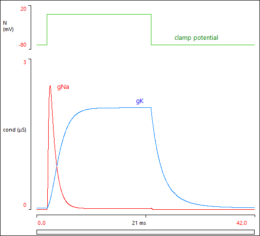
This shows the sodium and potassium channel conductances during a voltage clamp step from -70 mV (the resting potential) to 0 mV and back. This is typical of the data used by HH to construct their model. For convenience, the Results view is shown below:
gNa and gK. The conductance profiles during a voltage clamp step from -70 to 0 mV and back.
HH had already established the general voltage- and time-dependence of sodium and potassium conductance through experiments like those in the voltage clamp tutorial, but now they wanted to put it together to parametize their overall model. Specifically, they realized that by curve-fitting to the conductance profiles they could determine the likely number of voltage-dependent gates present in each channel type, and the time constant of the gate state changes at the clamp potential voltage. From this and a knowledge of the maximum conductance at the clamp potential, they could determine the opening (α)and closing (β) transition rate constants for the gates (see below).
Curve Fit in DataView
Neurosim does not have a general-purpose curve-fit facility, but the program DataView does. I am the author of that program, and it is available for free download here. To transfer the Neurosim results to DataView:
You can save the results in DataView format using the File: Export in DataView format: Save results to file menu command. However, for convenience, here is a link to a pre-saved file: HH vc cond.dtvw-dat. If you have DataView installed, then clicking this link should start DataView with the file loaded (although this may depend on your browser settings).
Further instructions in this tutorial section refer to DataView rather than Neurosim, unless stated otherwise.
Maximize the view showing the data within the DataView main window.
At this point you should see the three Neurosim traces displayed in DataView.
Select the Analyse: Non-linear curve fit menu command to open the Curve Fit dialog, and if possible move it so that it does not obscure the main view.
Potassium channel
In the Curve Fit dialog, set the Trace ID to 3 to load the K conductance trace.
The black curved trace is the conductance. The red trace is a line following the default linear equation, but ignore this for now.
Gate number and time constant
In their experiments data (just like in the Neurosim data here), HH noticed that the rising phase of K conductance had a distinct inflexion on it, while the falling phase looked more like a monotonic exponential. This underpinned their idea that the channel had multiple gates in it, all of which had to be open to allow conductance, but only one of which had to be shut to block conductance.
where gt is the channel conductance at time t after the step, g0 is the conductance at the immediate start of the step (t = 0) and g∞ is the steady-state conductance eventually achieved within the step. Note that the conductance values can be calculated directly from the data, but the n and τ values can only be obtained by curve-fitting. Also note that this equation can be applied to a voltage step in either direction, i.e. to the rising or falling phase of conductance, but we will start with the rising phase.
Use the Cursors: Place at time menu command to place a vertical cursor at 2.0 ms (i.e. just at the start of the voltage step).
Press the v key to place a second cursor in the middle of the view. This happens to be at 21 ms, which is towards the end of the voltage step and is appropriate for this analysis, but you could drag the cursor if you needed to shift its position.
The Curve Fit dialog now shows just the rising phase of K conductance. We now need to enter a suitable equation for an attempted curve fit to this trace.
Copy-and-paste the expression below into the Equation box in the dialog.
(a^(1/b) -(a^(1/b) - c^(1/b)) * exp(-t/d))^b
This is the same as equation \eqref{eq:eqNGatesRising}, but it has been put into a form suitable for curve-fitting in DataView. The parameter variables a, b, c and d refer to g∞, n, g0 and τ respectively.
The red line in the dialog now solves this equation, using the default initial parameter values shown on the left (parameters e - h are ignored since they do not occur in the expression). However, although the line is moving vaguely in the right direction, it is obviously a very poor fit to the data, and the fit process is likely to fail from this starting condition.
Click the Curve fit button.
The fit does indeed fail, with 2 error messages. The first just says which routine in the algorithm failed, and you can ignore this. The second suggests trying better initial parameters, and reducing the step size. Try the second suggestion first.
Click the Revert button to go back to the previous parameter values.
Change the Step size to 0.1.
Increase the Max iter to 150.
Click Curve fit again.
The red equation line gradually converges on the black data line as the parameter values change during the fit progression, and when the fit process terminates the two lines are almost identical. HOWEVER, there are two clues that not all is well. First, the fit algorithm ran for the full 150 iterations without converging (the delta value is still much bigger than the convergence criterion - press F1 for help if you want details on what this means). Second, and crucially, the b parameter value is very large and (probablyIf you add some noise to the conductance trace (as would be the case in a real experiment) you can also get a reasonable fit with a large positive exponent.) negative, which is physiologically impossible given the conceptual model on which the equation is based - it is vanishingly unlikely to have a huge number of gates and completely impossible for there to be a negative number of gates. The problem is that given the poor initial values, the algorithm has wandered off into a region of parameter space where there is a plausible (although not great) mathematicalfitI am actually somewhat dubious about the accuracy of the computational algorithm when calculating powers/roots this large, but that is another issue. to the data, but a completely impossible physiological fit.
The new a, c and d parameters (the ending and starting conductance, and the time constant) are plausible and provide quite good fits to the data, so we will use these are the new starting conditions.
Change b to 20 (i.e. plus 20, but you do not need the + sign)
This is a very high gate number so is probably wrong for the model, but provides nearly as good a fit to the data as the large negative value found previously.
Click Curve fit.
The fit converges after aboutThe fit algorithm does not always follow exactly the same value sequence on different runs from the same start. 100 iterations with a delta less than the convergence criterion, and the red fit line now superimposes almost exactly over the black data line, indicating a very good fit. The a and c parameters have only changed a little, but they now have almost identical values to those shown on the cursors, and the b parameter is very close to 4, which is physiologically plausible. It was this last datum that suggested to HH that there were 4 activation gates in the potassium channel. The d parameter is the time constant of the gate at 0 mV, and has a value of 1.530 ms (to 4 significant figures).
To see an alternative reality:
Set the value of b to 1, 2, 3 and 5 successively.
This shows what the conductance curve would have looked like if there were 1, 2, 3 or 5 gates in the potassium channel. The conductance curves with values of 3 and 5 are actually very close to that with 4, but remember that HH did this at multiple clamp potentials per axon, and replicated the experiment with several squid axons, so their concluded value of 4 was based on lots of data, not just one curve.
Now we will find the time constant for the falling phase of conductance.
We could move the cursors in the main view to bracket the falling phase of conductance, but the easiest thing is just to edit the timebase start time (the left-hand x axis scale) to 20 ms. This right-shifts the data display without moving the cursors, which now have e location times of 22 and 41 ms.
The black data line in the Curve Fit dialog should now show the falling K conductance.
Note that the right-hand half of the main display has run off the end of the data and displays all the traces in grey with a value of 0. These data are invalid.
Set parameter a to 0.1, b to 4, c to 2 and d to 5.
These provide a reasonably good starting point for the fit algorithm. (We could hard-code the b value as 4, since that was found from the rising phase, but it is useful as a reality check to allow the fit process to confirm this.)
Note: it might seem reasonable to have 0 as the initial "guess" value for a, since the conductance does decrease to almost 0. However, you should avoid this because the algorithm makes small positive or negative changes to the parameter values during fitting, and if a (or c) becomes negative, the algorithm will try to calculate the bth root of a negative number. For many values of b this will generate a not-a-number error, so convergence will be impossible.
Click Curve fit.
The b value is again very close to 4, but the key new information derived from the falling phase fit is the time constant at -70 mV, which is 5.458 ms.
Calculating α and β
To implement their model, HH needed to know the voltage-dependency of the opening (α)and closing (β) transition rate constants for the gates in the potassium channel. With a bit of algebra, they rearranged equations \eqref{eq:eqGateInfinity}
and \eqref{eq:eqGateTimeConst}
to get:
The root value 4 is the number of gates in the channel (derived from the curve fit earlier) and gv∞ can be measured from the voltage clamp data or the fit equation (for v = 0, gv∞ = 2.028). So what is now needed is the value of gmax, which is the maximum possible conductance when all the gates are open. This is a single value that does not change with voltage, and could be measured by running a very depolarized clamp step (assuming that this was enough to open all the gates), or, more realistically, by projecting the asymptotic conductance from a series of increasingly depolarized clamp steps. However, since we are working with simulated data, we can just look at the channel parameters in Neurosim, and see that the maximum potassium conductance is 2.827 μS for the simulated neuron.
We can now parametize equation \eqref{eq:eqNreCond} at a clamp potential of 0 to get:
which are indeed very close to the values of α and β for the potassium channel n gate at 0 mV.
Hodgkin and Huxley repeated these calculations for a whole series of voltage-clamp potentials, and then fitted the resulting α and β values to voltage-dependent Boltzmann-type equations, to generate the equations given at the beginning of this tutorial. And that was how they built their model for the potassium channel.
Sodium channel
Because the sodium channel inactivates, developing and parametizing a model for that channel was a lot more complicated, and I will only give a brief outline of some of the steps that HH had to undertake.
To make the problem tractable, they made a couple of (fairly heroic) simplifying assumptions: first that all the activation gates were shut at the resting potential (m0 = 0), and second that at steady-state there was complete inactivation at the clamp potential (h∞ = 0). This enabled them to produce this expression for sodium condutance (modifiedHH explicitly set m to 3. from equation 19 in their paper):
where g' is the steady-state value that sodium conductance would reach if h remained fixed at its resting level (h0).
Equation (\eqref{eq:eqM3Hgates}) can be written in form suitable for curve fitting in DataView thus:
a*(1-exp(-t/b))^d * exp(-t/c)
where a = g', b = τm, d = m, and c = τh.
Set the main view start time to 0.
Set the Trace Id in the dialog to 2.
You should now see the sodium conductance trace in the dialog.
Click the 1s button to reset the parameters.
Enter 3 and 0.1 for the a and b parameters respectively.
The Step size and Maximum iterations should be 0.1 and 150 from the previous fit - if not, set them now.
Click Curve fit.
The fit converges after about 100 iterations, and the red fit line closely follows the black data line over most of the plot. The d parameter, which represents the number of activaton gates, is closeProbably: see below for a discussion of exponent sensitivity. to 3 as per the HH model. The a, b and c parameters are 5.18, 0.21 and 1.05 respectively, and these values are very close to those that can be explicitly calculated using the HH formulae.
HOWEVER, the fitted value of the exponent d is very sensitive to the exact start time of the fit.
Drag the left-hand (start) cursor slightly to the left, i.e. earlier than the true start.
Click Curve fit.
The fitted d parameter is now (for my start time of 1.89 ms) close to 6!
Now drag it slightly later than the true start, and click Curve fit again.
With a start time of 2.07 ms, the best fit exponent is now close to 1.
It seems that with equation \eqref{eq:eqM3Hgates}, small changes in the start time can produce big changes in the best-fit exponent parameter. The other fitted parameters also change, but these changes are relatively small and stay fairly close to their explicit values. Note that if you make similar changes to the start time for the potassium conductance data using equation \eqref{eq:eqNGatesRising}, the exponent value stays close to the "true" value of 4. It is the added complexity of inactivation that makes the fit to equation \eqref{eq:eqM3Hgates} so sensitive. So this equation is not suitable for determining the number of activation gates, and HH did not use if for this purpose - they hard-coded the value 3 into their equation 19. However, curve-fitting to equation \eqref{eq:eqM3Hgates} does produce fairly robust estimates of the activation and inactivation time constants, and of the sodium conductance with a fixed inactivation level, and these are important components for deriving the α and β values as described previously.
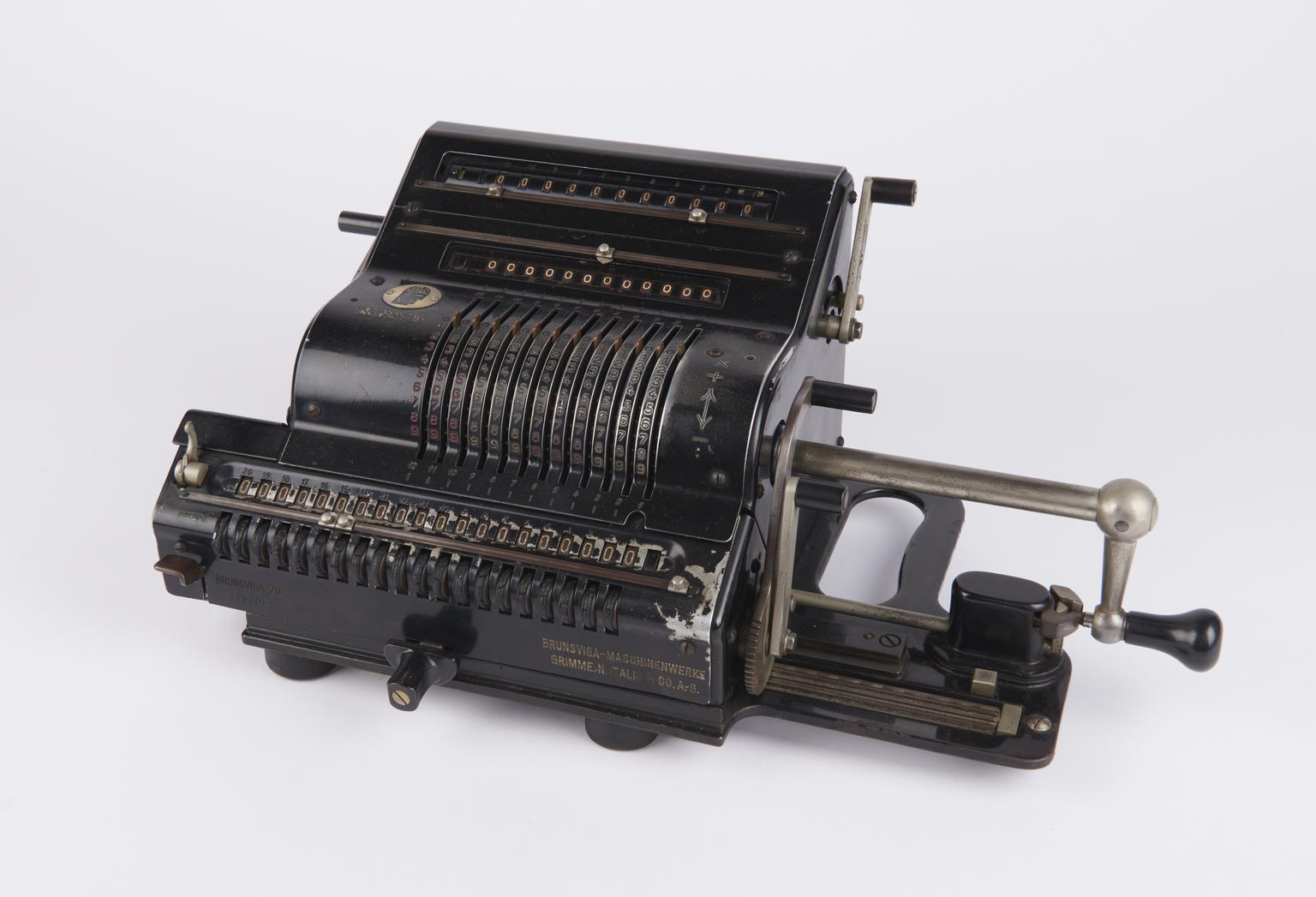
Finally, it is worth pointing out that HH explicitly state that their model and its parameters was entirely derived from the voltage-clamp data - they did not "retro-fit" any of the equations to produce realistic-looking propagating spikes with an appropriate threshold, a refractory period, rebound excitation, accommodation, or any of the other real-world phenomena that the model predicts with considerable quantitative accuracy. It is these "emergent properties" that make their model so impressive, and so useful. It has been estimated (Brown, 2020) that they must have carried out about 1 million individual calculations to derive their model and show its properties, and these would have been done using pencil and paper, slide rules, and mechanical calculating machines of the type shown below (purely for fun!). I think their Nobel prize was well deserved.
A key simplifying assumption of the HH equations, and one that is followed in most published research models, is that the current flowing through ion channels can be described by a modified version of Ohms Law - the driving force equation (\(I=g(V_{m} - V_{eq})\)), and that the core channel conductance when all gates within it are open has a fixed value (gmax). This implies that any changes in channel conductance are due to the opening and closing of the voltage-dependent gates within it.
However, this is usually not exactly true. If there is an imbalance in the concentration of the carrier ion on either side of the membrane, then the core channel conductance will almost certainly rectify – it will have a higher conductance in the “downhill” direction of the concentration gradient than in the “uphill” direction. This follows from basic physical chemistry (there are more ions available to carry current from high to low concentration than vice versa), and Hodgkin and Huxley were well aware of it. They were able to ignore it because the effect is quite small in the voltage and concentration ranges with which they were dealing. However, if the concentration ratio is large, the effect can become significant, and it may be better to use a more sophisticated model of channel conductance based on permeability. This involves the Goldman-Hodgkin-Katz (GHK)currentThe GHK current equation underlies the GHK voltage equation, which we have come across before in the calculation of the resting potential. equation, which is an equation based on electro-diffusion theory that calculates the current flow across a membrane given the voltage, permeability and ion concentrations:
In this equation i is the current density carried by the ion in question, [in] and [out] are the intracellular and extracellular concentrations of the ion respectively, P is the membrane permeabilityPermeability, unlike conductance, is a fixed value that is independent of ion concentration. of that ion, V is the membrane potential, z is the charge (valency) of the ion, R is the gas constant (8.314 J K-1 mol-1), F is Faraday’s number (96485 C mol-1), and T is the absolute temperature (294°K).
In Neurosim, the equation assumes that the user-specified value of P is relative to 1 cm2 of membrane, and during the calculation it is scaled by neuron surface area to produce an absolute current. Calculating the GHK equation is considerably more time consuming than calculating the standard driving force equation, which is why computational models avoid using it if possible.
Rectification
It is clear from the equation \eqref{eq:eqGHKCurrent} that for a constant voltage, the trans-membrane current is dependent on the absolute ion concentrations on either side of the membrane, and the difference between those concentrations. This means that the channel does not obey Ohm’s Law.
The initial result shows the membrane potential change induced by a negative current pulse, and at this stage it looks much like the response of a standard RC circuit.
Double-click the GHK channel in the Channels list in the Setup view, to open the Voltage-Dependent Channel Properties dialog.
Next, note that the Use GHK current option is selected (towards the bottom-left of the dialog). The carrier ion is unspecified, but it is positively charged and monovalent (z = +1), and the intracellular concentration is much higher than the extracellular concentration.
In the Setup view, click the up-arrow of the stimulus Pulse 1 Amplitude, to increase it to -1.5 nA.
As you would expect, the smaller stimulus produces a smaller voltage deflection.
Without clearing the screen, repeatedly click the up-arrow until the stimulus reaches +2 nA.
It should be clear that the largest positive current stimulus produces a smaller voltage deflection than the equivalent-sized negative current stimulus. Remember, for a given current, a smaller voltage response implies a larger conductance, so the result shows that it is “easier” for a positive current to push the positively-charged carrier ion out of the cell (down its concentration gradient), than for a same-sized negative current to pull it into the cell (up its concentration gradient). This is rectification.
Task: Construct a graph showing the relation between stimulus current and voltage response (a classic I/V curve).
Check the Measure box in the Results view.
Drag the vertical cursor slightly to the right into the region within the stimulus where the voltage has completely stabilized.
Click the Measure button in the Measure dialog.
Click Plot in the Measure dialog.
Select Voltage from the drop-down list for the X axis, and Stimulus from the drop-down list for the Y axis.
If the response was Ohmic as in a classic RC circuit, the plot should be a straight line, but in fact it curves upwards on the right. A curved I/V plot is a diagnostic feature indicating rectification.
GHK and Leakage Currents
In this experiment, the current is passing through two channels – the GHK channel, and the standard leakage channels, the latter of which in Neurosim are Ohmic in their response. To separate these effects, we need to switch to voltage clamp mode.
Without clearing the screen, click the up-arrow of the Clamp 1 potential to increase it by 10 mV.
Note that there is a rather small change in the GHK current, but a bigger change in the leakage current.
Repeatedly click the up-arrow of the Clamp 1 potential until it reaches -40 mV.
As the voltage increases, the current step in the GHK channel (red trace) also increases.
This again indicates rectification in the GHK channel -
equal-sized voltage changes would produce equal-sized current changes in an Ohmic conductance. The latter can be seen in the leakage current (green trace), where each current step is of equal size.
Task: As before, construct an I/V plot of the voltageversus current changes, but this time switch the Y axis selection between the leakage current (I Leak) and the GHK channel current (I Chan 1), and compare the two plots.
The leakage I/V plot should be linear, crossing the 0 current intercept at -60 mV. This is consistent with the leakage equilibrium potential of -60 mV (you can open the Passive Properties dialog to check the settings if you wish). The GHK I/V plot is curved, indicating rectification. It does not cross the current intercept because the GHK equilibrium potential is more negative than any voltage in the experiment. (It is actually -192.6 mV, as can be seen in the Channel Properties dialog which uses the ion concentration ratio to calculate the Nernst potential.)
Take-home message: Real ion channels are often rectifying – they conduct current more easily in one direction than the other. This arises naturally if there is a difference in the concentration of the carrier ion on either side of the membrane. However, the effect is usually small, and can be ignored in most simulations.
The GHK current equation provides a more sophisticated description of channel behaviour than the standard Ohmic model. However, it too has limitations. An assumption underlying the equation is that ions move completely independently of each other, whereas in fact many channels act like narrow tunnels in which ions cannot move past each other. It also assumes that the membrane is homogeneous, with a uniform electric field and a uniform ion concentration gradient within the membrane, which is probably not true for proteinaceous channel pores. So although the GHK equation might be (somewhat) more accurate than the standard driving force equation, it is certainly not the last word on the matter!
Conductance
In a GHK channel the permeability is specified, but not the conductance. Neurosim calculates and displays an effective conductance by “reverse engineering” the driving force equation. This yields what is known as the chord conductance (see Thompson, 1986 for a detailed discussion of chord and slope conductances), which is analogous to the conductance used in the HH equations. However, the conductance value can be inaccurate if the membrane potential is close to the equilibrium potential because then the calculation involves dividing a very small current by a very small driving force. If the membrane potential is actually at the equilibrium potential, the conductance cannot be calculated due to a divide-by-zero singularity (avoided in the simulation by offsetting the membrane potential slightly).
Morris-Lecar: Reduced Kinetics
So far we have been looking at the Hodgkin-Huxley model and various complex elaborations developed from it. However, a very influential model has been one that reduced the complexity - the Morris-Lecar model (Morris and Lecar, 1981).
The simulation implements the model with the kinetic parameters specified in the original paper, which were based on muscle fibres in a barnacle. A stimulating current is applied to reproduce the behaviour shown in Figure 6 of that paper.
The spikes do not look very “convincing” in terms of what we expect nerve spikes to look like, but the important point about this model is that it produces spike-like behaviour from an extremely simple basis. There are only two channels, one with a depolarized equilibrium potential, nominally a calcium channel, and the other with a hyperpolarized equilibrium potential, nominally a potassium channel. Each channel has just a single gate, and neither channel inactivates. The spike-like behaviour arises purely from the activation kinetics of these two channels.
Double-click the Ca channel in the list to show its properties dialog.
Check the Show graph box just below the Equations choice options in the dialog.
The calcium activation curve has a mid point at 0 mV (note the v – 0 component in the user defined equation – the 0 is obviously unnecessary here, but it indicates where the mid-point parameter would be placed if it were non-zero), which is very depolarized. But so is the resting potential of the cell (-50 mV), and it takes a depolarizing stimulus to activate spikes.
Change the channel ID (top left-hand corner) to 2, to look at the K channel kinetics.
The activation curve moves slightly to the right (note v – 10 in the equation). This means that the potassium channels open at an even more depolarized membrane potential than the calcium channels – they will open after them as the membrane depolarizes in response to the stimulus.
Change the Channel Properties graph Display to Time Constant.
Note from the graph Y-scale value that the time constant peaks at 10 ms. Also note the factor 0.1 which multiplies the cosh in the equation.
Uncheck the Autoscale Y box in above the graph (this will show changes more clearly).
Switch back to channel ID 1 (the Ca channel).
Now the maximum time constant is only 1 ms (the 0.1 cosh factor in the equation has disappeared). So not only does the calcium channel activate at a lower voltage than the potassium channel, but also it activates much more rapidly. This is an example of a so-called fast-slow model, where there are just 2 simple channel types, but with a significant difference in the time-scales at which they operate.
Equations
The user-defined equations involve terms which may be unfamiliar – the hyperbolic tangent and cosine functions (tanh, cosh). However, the equations could be re-written in exponential form to give similar results.
With channel ID 1 selected, and the Probability Display showing on the graph, select the Pre-defined inf/tau equation option which involves exponentials.
The time-infinity activation curve does not change at all with the parameters chosen for the pre-defined equation. You can switch back and forth between the Pre-defined and User-defined equations with no change.
Further reduction
Solving the Morris-Lecar model requires integrating 3 differential equations: one for m, one for n, and one for V. This is in contrast to the full HH model, which requires solving 4 differential equations (\eqref{eq:eqGrandHH1} - \eqref{eq:eqGrandHH}) (the additional one is for h). However, the calcium channel gate time constant is very short. What happens if it is removed altogether?
Click Clear in the Results view.
In the Voltage-Dependent Channel Properties dialog for the calcium channel, set the Time constant equation to 0.
Click Start.
Note that the system still responds to the stimulus with a train of action potentials. The frequency and shape of the spikes is somewhat different, but essentially the system behaviour is unchanged when the short time constant is eliminated completely.
By removing the time-dependence of m we have made it an instantaneous function of voltage, and its value no longer has to be calculated by integrating a differential equation. It can be calculated explicitly just by solving the Infinity value equation at the required voltage. This means that the reduced Morris-Lecar model only requires solving two differential equations.
Significance
The significance of the reduced Morris-Lecar model lies mainly in its mathematical tractability as a dynamical system with just two differential equations. Such systems are amenable to a technique called phase-plane analysis, and there have been numerous papers published which use this to explore the properties of this system. This is discussed further in the next section.
Take-home message: The Morris-Lecar model uses the HH formalism but with fewer parameters. It produces spikes with just two single-gate non-inactivating voltage-dependent channel types, a fast depolarizing channel and a slow hyperpolarizing channel. The reduced form of the model involves only 2 differential equations, and is highly amenable to mathematical analysis.
Phase Plane Analysis
The original Hodgkin-Huxley model is a dynamical system described by a set of four coupled differential equations with state variables m, h, n and v \eqref{eq:eqGrandHH1} - \eqref{eq:eqGrandHH}. These variables change with time, and normal analysis and display involves plotting them (or dependent variables such as conductance or current) against time itself. That is what most of the displays in Neurosim show. However, if the variables are plotted against each other rather than against time, the result is a plot in phase space.
A plot with 4 dimensions is virtually impossible to display graphically, and equally difficult to analyse. However, if the system can be described by differential equations involving just two variables, then it is easy to make a phase plane plot on a 2D surface like a computer monitor (or, in the old days, a sheet of paper ...).
Why would one want to do that?
First, there is a very well developed set of mathematical procedures that can analyse the properties of just two coupled differential equations. This analysis can tell whether the system is stable, multi-stable, prone to regular oscillation, chaotic, explosively unstable etc. The other advantage of a phase plane plot is simply that it gives an alternative view of the shape of the system response, which can emphasise features that are not immediately obvious in a normal time-series plot.
The mathematical analysis of phase plots is beyond the remit of this tutorial (and the expertise of this author), but Neurosim can produce phase plane plots that give a qualitative flavour of the methodology.
The key point about this model is that it is driven by just two differential equations. There is an equation that specifies the voltage that operates on a fast time scale, and another that specifies the open probability of the potassium channel that operates on a slow time scale.
Select the Analyse: Phase-Plot menu command to show the Phase Plot dialog. Move the dialog so that you can also see the Results view.
In the Phase Plot dialog, select Voltage from the Y axis drop-down list, and Prob chan 2 gate 1 (i.e. the n gating variable of the potassium channel) from the X axis drop-down list. This will plot the two state variables of the equations against each other when you run the simulation.
[
Remember that the m gating variable of the calcium channel is an instantaneous (although non-linear) function of voltage, so plotting against voltage is functionally equivalent to plotting against m.]
Click Start and observe the plot, although it probably develops too quickly for you to see details.
When the simulation finishes, select Autoscale for the X and Y axes to enlarge the plot.
Unless you have a rather slow computer, select a Slow down factor (perhaps 3) from the drop-down list in the main toolbar.
Click Start again. This time the simulation runs more slowly, and you can watch the plot develop.
As the simulation progresses, you should see the plot trace a clockwise trajectory around the graph, with each spike generating an individual loop.
(If you have selected too large a slow-down factor and you get bored, you can reduce it on-the-fly during the simulation.)
While the simulation runs, the plot is black-and-white, but when it terminates it is colour-coded by time. This can be seen more clearly in a 3-D graph.
Click the 3-D button in the Phase Plot dialog to open a 3-D display of the plot
Select Auto Y in the Rotation group of the 3-D graph.
You can also select Mouse, and drag the plot manually to change the viewpoint.
As the plot rotates, you should see that the plot trajectory forms a helix, with the blue end being the start of the simulation (time 0) and the yellow end being the end (time 800 ms).
So what does all this tell us? The first and probably most important point is that the repeating loops in the plot form what is called a limit cycle, and limit cycles are characteristic of oscillating dynamical systems. The limit cycle can be understood by following through the various stages as follows.
Click None, followed by Default in the Rotation group of the 3-D graph. You may also want to expand the size of the dialog to see things more clearly.
At the starting point (blue end of the helix) the membrane potential (Y axis) is low, and so the open-probability of the n gates (X axis) is also low. This positions the starting point towards the bottom-left of the graph.
As the membrane depolarizes during the rising phase of a spike the graph trajectory rises due to the increasing value of the Y variable (voltage).
However, the potassium conduction is slow to react to changing voltage and so is still low at this stage. So the graph trajectory remains on the left-hand side of the plot reflecting the low open-probability of the n gates.
Once the spike gets close to its peak, the n gates tend to open, and the graph trajectory moves to the right due to the increase in value of the X variable.
The increased potassium conductance caused by the opening n gates causes a fall in membrane potential, so the graph trajectory moves downwards, starting from near the top-right of the plot.
As the membrane potential hyperpolarizes, so the open-probability of the n gates decreases, causing the graph trajectory to move diagonally downwards towards the left (decreasing Y and X values). This brings it back towards its starting point (the actual starting point is before the stimulus starts, so is more negative than the lowest part of the limit cycle oscillations).
Then the cycle repeats for the next spike.
When the stimulus switches off, the membrane potential again drops to its resting value (the yellow end of the helix).
Close the 3-D plot when you are ready to move on.
To further examine this, what happens if there are no spikes, or if spikes fail?
In the Phase Plot dialog, uncheck the Autoscale X and Y boxes, so that the plot does not change scale.
Set the Slow down factor back to 0 - you know how the plot develops, so don't need the visual clues.
In the Setup view, set the stimulusamplitude of pulse 1 to 2 nA.
The stimulus is now below threshold so no spikes are generated. The membrane potential rises and then falls as the stimulus occurs, but the open probability of the n gates does not significantly change in this voltage range. Consequently, the phase plot is just a vertical line, with no sign of a limit cycle.
Set the stimulus amplitude to 2.5 nA. This is close to threshold, and sometimes the noise takes the membrane potential above threshold.
Click Start a few times, and observe the dramatic change in the phase plot when spikes occur.
There can also be spike failure due to excessive stimulation. To see this most clearly we need to remove the noise.
In the Setup view, check the Passive box in the Cell properties group to open the Passive Properties dialog.
Set the Noise amplitude (the bottom edit box) to 0.
Click OK to close the dialog.
Set the stimulus amplitude to 7 nA.
The Results view shows spikes failing due to massive activation of potassium channels. The phase plot shows the limit cycle spiralling inwards to a single point, called a stable focus.
Open the 3-D dialog again to see this most clearly.
You may want to check the Autoscale boxes to keep the plot within the axis limits.
The 3-D plot trajectory has a conical shape that tapers to a straight line in the Z (time) axis, reflecting the focus in the 2-D plot
Take-home message: Dynamical systems with stable oscillations show a limit cycle (a circular trajectory) in the phase plane. If the oscillations are not stable but fade out, the limit cycle will spiral in towards a stable focus.
Phase Plots of Experimental Data
The main use of phase plots in computational neuroscience is for the mathematical analysis of model systems, where the analyst has access to the state variables of the underlying equations. However, in experimental neuroscience, phase plots are also quite commonly used to present an alternative visualization of a system response.
In these cases, it is usual to plot the slope of the membrane potential against the potential itself (i.e. dV/dt against V).
We don't have real experimental data in Neurosim, so we will just use an HH spike instead.
Load and Start the parameter file Hyperkalaemia. This featured in an earlier tutorial examining the unfortunate effects of excess extracellular potassium.
Activate the Phase Plot dialog with the Analyse: Phase Plot menu command.
Note that the default axis selection is dV/dt and Voltage, which is what we want.
Nothing is visible in the plot at this stage, because with no change in membrane potential, the data form a single pixel.
In the Setup view, click the up arrow of the extracellular K edit control.
A single spike shows in the Results view, and the Phase Plot shows a limit cycle similar to what we saw previously.
In the Results view, click the expand timebase button in the toolbar () four times, so that the right-hand timescale reads 12.5 ms (you could actually also just set this value explicitly).
Task: Bearing in mind that the phase trajectory moves in a clockwise direction, work through how the phase plot arises from the voltage profile of the spike in the Results view. Here are some questions to help you focus:
Questions:
What does the highest point on the trajectory in the phase plot graph represent? Where does it occur on the spike itself?
What does the right-most point represent? What is the value of the voltage derivative at this point, and why? (You can get a read-out of values by hovering the mouse over the plot.)
Which part of the phase plot is generated during the after-hyperpolarization? To answer this, you may want to re-run the simulation with a large slow down factor, so that you can follow the trajectory.
The answer to this last question illustrates how a feature that may occupy a large part of a plot in time-domain visualization, may almost disappear in a phase plane visualization.
Now let us further increase the extracellular potassium concentration.
Set the slow down factor back to 0 if you changed it.
Click the up arrow on the potassium concentration to change it to 14 mM, and observe what happens.
Repeatedly click the up arrow, until you reach a concentration of 32 mM.
The limit cycle rapidly collapses into a stable focus. Which is pleasing visually, but would, of course, be disastrous in a biological system.
 ) and drag across the current spike to zoom in on it.
 ) to return to the full display.
 ) in the Results toolbar to zoom in on the spike a bit.
 ) in the Results toolbar.