Tetrode (n-Trode) Spike Sorting

It is increasingly common to make extracellular recordings using multiple monopolar electrodes whose recording tips are very close to each other (maybe only 10's of μm apart). The electrodes are physically bundled together and move as a unit, so they maintain the same spatial relationship to each other as they are moved. Four such electrodes are known as a tetrode, but in principle, and increasingly in practice, there can be more than 4 electrodes, leading to an n-trode.

The advantage of an n-trode is that each electrode records from adjacent but slightly different regions of extracellular space. This means that axon A might be close to electrode 1 and thus produce a big spike in its trace, while producing a smaller spike at electrode 2 because it is slightly further away from it, and no spike at all in the traces from the other electrodes in the bundle. Axon B, on the other hand, might be close to electrode 2 and produce a big spike there and a small spike in electrode 1. And so on. The point is that the regularity in the differences in waveforms recorded at the various electrodes gives a lot more information about the identityIt can also give information about the spatial geometry of the axons relative to the electrode, but that is not part of the tutorial. of the axons generating the various potentials than can be obtained from a recording made by a single electrode.

DataView provides a fairly simple method for spike sorting from n-trode recordings using simultaneous principal component analysis (PCA) from all, or a sub-set, of the electrodes. There are more sophisticated packages available (e.g. Pouzat & Detorakis, 2014), but the "off-the-shelf" procedure described here is often suitable for an initial analysis.

• Load the file 3-trode.

ThisThe file was kindly supplied by Dr Judith Schweimer, University of St Andrews. shows 3 traces from a tetrode implanted in the brain of a freely-moving mouse. Visual inspection shows that there are more spikes visible in the top trace 1 than the others, so this will be taken as a "master" trace for analysis. The first task is to detect spikes in this trace.

• Select the Event edit: Threshold menu command to open the Threshold dialog.
  • Select -ve as the Threshold Onset parameter. This is most suitable because the spikes have a larger negative than positive deflection.
  • Select Med +/- rob sd x mult as the Threshold source, and Whole file as the Trace stats source.
    This means that the threshold level is set objectively as a multiple (5 by default) of the robust standard deviation of the entire recording in trace 1.
  • Click Analyse, and note that 89 spikes are detected.
  • Close the Threshold dialog.

We need to adjust the events to encompass just the spike waveforms.

• Activate the Event analyse: Event-triggered scope view menu command to open the Scope view.
• Set the Count to -1 to show all 89 sweeps.
• Set the Start (re-trig) to -0.25 and the Sweep dur to 1.25 ms.
  The Scope view now shows a window that is focussed on the spikes and is suitable for PCA.
• Click the Ev = Disp button near the centre-top of the view dialog.
  This adjusts the timing of all the events in channel a to match the data visible in the Scope view.
• Select the from Events option in the Sweep colours group.
  This turns all the sweeps black, which doesn't help at the moment, but will be useful later.

The spike-like waveforms in the top trace seem to form a single size cluster with rather a wide amplitude distribution, with an additional group that may be spike-generated (it has a dip in the middle), but may also be just random noiseThe "noise" may of course be caused by spikes in multiple axons which are distant from the recording electrodes and thus whose small field potentials merge into an indistinguishable "mess" of waveforms. that happened to cross the threshold (remember that all the waveforms in trace 1 must have a negative phase that crosses the threshold, or they would not generate an event and would not display in the Scope view). However, the waveforms in the lower 2 traces seem to fall into 2 size clusters in each, although the smaller tends to merge with the putative noise. The aim is to separate these into the different combinations in which they occur.

• Move the Scope view to one side if possible, but leave it open.
• Select the Event analyse: Shape classification/clustering: Principal component analysis: N-trode menu command to open the PCA and Clustering dialog.
• Click Calculate to calculate the first 3 PCA coefficients for the selected trace 1.
  There appear to be 2 groups (clusters) in the 3D graph that becomes populated by the coefficients.
• Click the Cluster button in the PCA dialog to activate the Cluster dialog, and then click the Cluster button in that dialog to cluster the coefficients.

There are indeed 2 clusters in the PCA coefficients from trace 1 displayed in the 3D graph in the PCA dialog. One (coloured red) represents the spikes, the other (coloured cyan) the noise. Note that the sweeps in the Scope view showing spikes now show in the same colours as their PCA coefficients, i.e. the spikes are red, the noise is cyan. However, all the spike types in each of the 3 traces are coloured red and thus belong to the same group. Clearly, PCA on spikes in trace 1 alone does not separate out the different spike combinations in the tetrode recording.

• Cancel the Cluster dialog, and note that the sweeps in the Scope view all return to a black colour.
• In the PCA dialog, change the Traces edit box to show "1 2 3".
  The 3D graph of coefficients clears when you change the source trace.
• Click Calculate again to get revised estimates of the first 3 PCAIf you click the % var button you will see from the Eigenvalue list that these account for > 92% of the variance. You may be tempted to include more PCs in the analysis, but in fact this degrades the clustering algorithm used next, which fails to "see the wood for the trees" if presented with too many dimensions containing similar information. coefficients.

With all 3 traces selected, PCA is performed on the concatenated waveforms of the 3 traces underlying each event. This thus detects different patterns in the combinations of the 3 trace waveforms, not just patterns within a single trace. There are now 3 clear groups in the coefficient graph.

• Click the Cluster button in the PCA dialog again to activate the Cluster dialog, and then again click the Cluster button in that dialog to cluster the coefficients.

There are now 3 clusters detected, coloured red, cyan and blue. As before, the sweeps in the Scope view are coloured to match the cluster within which they occur.

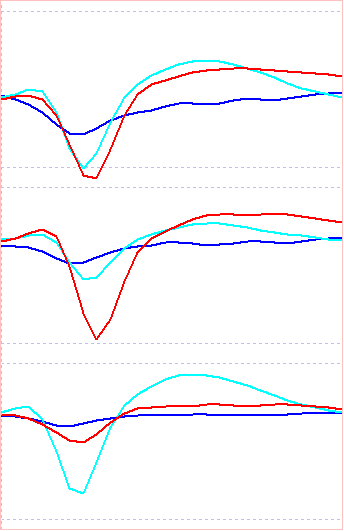
• In the Scope view, check (and then uncheck) the Avg box in the Average group. This displays the point-by-point average of the sweeps in each colour group in each trace.

a

b

c

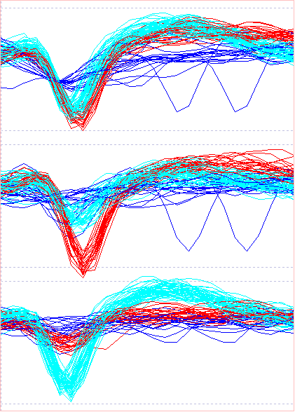
What does all this mean?

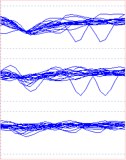
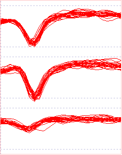
The Scope view shows that blue represents the putative noise in all 3 traces, while the red and cyan traces are generated by spikes in 2 different axons. In trace 1 the red and cyan spikes are intermixed - their traces largely overlap and do not fall into 2 obvious groups. In trace 2 the red spikes are clearly separate, but the cyan spikes merge continuously with the blue noise . In trace 3 the cyan spikes are clearly separate, but the red spikes merge continuously with the blue noise. Thus if a recording had been made with a single electrode in any one of the 3 locations it would not be possible to distinguish the 2 separate spikes. The 3-trace recording from the tetrode allows this separation.

• Click OK in the Cluster dialog to lock in the colour changes and dismiss the dialog.
• Click Partition in the PCA dialog, then OK in the Partition dialog to accept the defaults.
• In the Scope view, scan through event channels b, c and d to see the different waveforms of the noise, red spike and cyan spike as recorded at the 3 different electrodes.

a

b

c

The sort of axon-electrode spatial relationship that could produce this recording is shown below:

	Ax A		Ax B
E 2		E 1		E 3

Caveats

The recording used for this tutorial is particularly "nice" because it contains spikes from 2 axons that are large but indistinguishable from each other in trace 1, while one produces a large spike in trace 2 but not trace 3 and the other produces a large spike in trace 3 but not trace 2. This means that they can be separated from each other with a single spike-detection procedure using trace 1 as a master trace. However, it is not always so simple. It could easily be the case that there was another axon that produced a prominent spike in trace 2 and/or 3, but no spike in trace 1. This would not be picked up by the single analysis described above. In such a case it would be necessary to detect spikes in trace separately, and then merge events from spikes common to multiple traces.

 

---