Hill-valley analysis

The purpose of hill-valley analysis is to mark relevant peaks in a recording with events, while ignoring irrelevant peaks. The latter may be small lumps and bumps produced by genuine but irrelevant signals, or simply noise.

Open the file hill-valley.

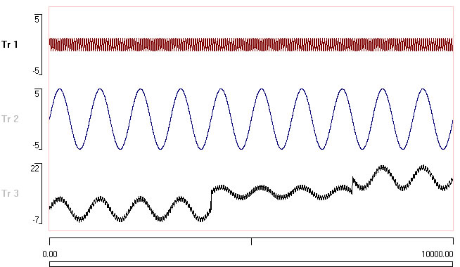
The upper trace shows an extracellular recording from the abdominal first root of a crayfish displaying swimmeret activity. The lower trace shows the data after de-meaning, rectifying and smoothing with 4 iterations of a moving-average filter with a half-window of 50 ms (Transform: De-mean/median, rectify, smooth). This transforms the spike data into a series of rolling hills and valleys.

Select the Event edit: Hill-valley analysis menu command.
In the Hill-Valley Analysis dialog box, set the trace to 2 and look at the preview in the bottom-right of the dialog. The red boxes at the top show the events that would be detected with the current settings.

Hill valley analysis — The Hill-valley analysis dialog preview. Hills (h) and molehills (m) have been marked, and molehills may occur either on the uphill (u) or downhill (d) slope of an adjacent hill. The designation is determined by whether the rising slope (r) is less than the falling slope (f), making a downhill molehill, or *vice versa*.

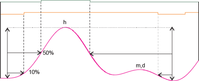
In these data, peaks can be subjectively divided into “hills” reflecting the main bursts, and “molehills” reflecting antiphasic interburst activity. Furthermore, if the rising slope of a molehill is shorter than the falling slope, the molehill must be occurring on the downhill slope of a preceding hill (see inset), while if the falling slope is shorter than the rising slope, the molehill occurs on the uphill slope of a following hill. Molehills that are actually deflections on the slope of a major peak are referred to as “foothills”.

The default parameters simply detect every peak in the selected trace, and mark them with events that start half-way up the rising slope and end half-way down the falling slope due to the Threshold setting of 50% (see the last peak in the image above). The data within each event are drawn in red. The troughs and peaks are connected by straight blue lines in the preview.

The preview only shows data visible in the main view. However, the dialog is non-modal, so you can navigate through the file to look at different sections if you wish.

Click the Left page toolbar button () in the main view.

You now see a different set of peaks in the preview (and different data in the main view). Note that the right-most peak in the preview is not marked. This is because there is no detectable trough (valley) on its right. To be detected, each peak has to have a trough on either side of it.

Click the Right page toolbar button () in the main view to return to where you started.
To actually insert these events, click ANALYSE at the bottom left of the dialog.

The default for the dialog is only to analyse the data visible in the main view (this is to reduce the chance of accidentally analysing a huge file, and needing to go for lunch while this happens). However, you can change that by selecting a different choice in the Analysis window frame.

To refine the analysis, you can filter the data by both height and duration. Any non-zero filters are displayed as coloured bars in the bottom-left of the preview, to provide a visual key to their values.

Height filter

There are 3 molehills in the displayed data, and you may want to get rid of them since they are generated by anti-phasic activity (which we will assume is irrelevant). This can be done using the Height filter options near the bottom-left of the dialog.

The easiest interactive way to set a filter is by dragging with the mouse. However, you can also set filter values explicitly in the edit boxes, or by dragging cursors in the histogram or preview windows. You can also set the values as multiples of the standard deviation (robust or normal) of the appropriate parameter.

If multiple filters are selected, they are performed in the following order.

Merge foothills

Click the Drag button in the Merge foothills row in the Height filter frame, and drag a box in the preview from the peak to the trough of one of the larger foothills.

A blue bar appears in the preview, indicating the value of the filter.

To make sure that you get the same result as this tutorial, now set a value of 5 in the Merge foothills box.
The blue bar probably changes in height, but unless you dragged over an inappropriate distance, the result should be the same.

The result is to merge foothills (molehills) with their associated hill (preceding or following, see above). You can see this in the change in the blue lines connecting peaks and troughs in the preview. The foothill peaks fall under a straight section of the blue line because they are merged with the adjacent hill.

The resulting events depend strongly on the Event threshold setting.

Note that with the default 50% setting, only the main peak is encompassed.
Change the up and down thresholds to 10%, and observe that both the main peak and the foothill are now within the event (see image below).
Change both thresholds to 100% and note that a point process event would now be placed at the peak of the hill.

Merge foothills — The threshold setting affects the duration of the events marking the hills. The analysis is performed after merging the foothill (m,d).

With some threshold values the event duration is potentially ambiguous:

Set both the up and down thresholds to 15%.

Note that the molehill is excluded from the event. This is because by default the event starts and finishes when the trace value crosses the specified percentage measured from the centre (peak) of the event.

Select edges from the measure from options.

Now the molehill is included in the event, so there is a step increase in event duration. The difference is because threshold in the merged hill is crossed twice - once on the downhill slope of the main peak, and again on the downhill slope of the molehill.

Set the Event threshold values back to 50%, and the measure from choice to centre.

Note that iIf there are several foothills surrounding a peak, then they are merged consecutively until the overall hill exceeds the threshold criterion. We will see this in detail in the Complex analysis section below.

Histogram

Above the preview there is a histogram showing the frequency of heights in the preview data. The 3 molehills are visible as the 2 sets of left-most bars (uncheck the Ln Y option to see actual counts in a more readable way). When you set the Merge foothills above 0, a blue vertical cursor appears in the histogram. You can drag this to adjust the parameter interactively with immediate feedback, if you wish.

With the default Relative ht (raw) selected as the histogram Show option, the heights of the shorter slope of all peak-valley combinations in the preview raw data are shown. These do not change with filtering. If you select Relative ht (merged), the heights after the merge filter are shown. These can change as you change adjust the filter.

Exclude molehills

Return the Merge foothills value to 0 and
Set the Exclude molehills value to 5.

With these data, the resulting events are identical to those achieved with the Merge method. However, if you look at the blue lines connecting peaks and troughs, you can see that the molehills are not merged with their dominant adjacent hill but still recognized as hills in their own right (they have their own blue lines peaks). However, they are not marked by events - they have been completely excluded .

With different data, or with different Threshold settings, merging and excluding can produce different results.

The exclude threshold shows in the histogram as a brown cursor, and this too can be dragged.

Absolute threshold

There is a dark green draggable horizontal cursor located near the bottom of the preview. This indicates an absolute threshold - peaks have to cross this to be counted.

Rset both Merge foothills and Exclude molehills back to 0.
Drag the green cursor upwards so that only the large peaks rise above it.
The Absolute threshold filter value probably reads about 45 - set it to 52 by directly editing its value.
Now only 3 hills are detected, because only these 3 have a peak amplitude above 52.

Objective threshold values

The height filter settings can obviously have a major impact on the detection of hills in lumpy data. It would be nice to have an objective method for setting such values, rather than relying on "by eye" judgement. One way to do this is to measure characteristic values, such as maximum peak-to-peak deviations, from a section of "quiet" data. Since the Hill-Valley Analysis dialog is non-modal, such measurements can be made and tested seamlessly while keeping the dialog open. However, there are also some objective options built in to the dialog.

Load the file robust hills.

There are 3 very obvious hills in this constructed data, but because random noise (mean = 0, s.d. = 1) has been added to the trace, there are numerous molehills which are detected with the default settings. Since noise is frequently present in data, this is a common problem.

Check the use SD x in box the Exclude molehills row of the Height filter group. (Using Merge foothills would do equally well in this case.)

This action sets the Exclude molehills threshold to 5 timesIf desired, you could adjust the multiplier by changing the 5 in the adjacent edit box to another number, but 5 is often a suitable choice. the robustThe robust standard deviation is 1.4826 times the MAD (median absolute deviation from the median). standard deviation of the shorter of the two slopes on either side of each hill. The statistic is measured from data within the Analysis window (which in this case is the visible screen, which is also the whole file). A brown vertical line appears in the preview indicating the height of the threshold filter, and the actual value is shown in the edit box as 4.4 (the edit box is now read-only).

Now only the 3 obvious peaks are marked as hills, which is what we want.

If you wanted, you could use the normal standard deviation rather than its robust version:

Uncheck the robust box near the top of the Height filter group.

The filter threshold is now much larger, and all the hills are excluded, including the ones that we wanted to detect. The reason is that the 3 big peaks have a very strong influence on the normal standard deviation - they make it much larger than that generated by just the added noise. The robust standard deviation is much less influenced by such outliers.

Click the Stats button in the Analysis window frame.

The results shows a variety of statistical measurements that can be used to set threshold values objectively, if the built-in shorter slope option is not suitable. But for now, note the difference between the normal S.D., which is nearly 6, and the robust S.D., which is close to 1. The latter reflects the added noise (which does indeed have a S.D. of 1) more accurately.

Duration filter

Once the data have passed through any height filters, they can be filtered by duration. You can set both a Minimum and Maximum duration, and any events which do not meet these criteria are excluded.

Select Duration as the Show option in the histogram to see the frequency of event durations. Again, there are draggable cursors enabling interactive parameter adjustment.

Complex analysis

The various filter options described above allow suitable hills to be detected in quite complex data.

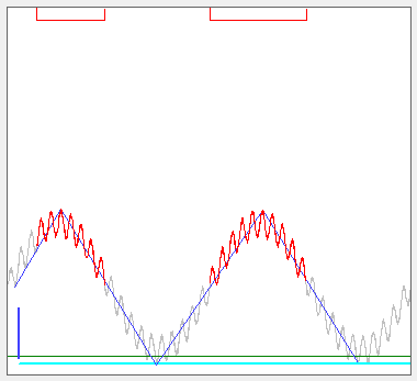
Load the file lumpy sine princess.

The top trace contains a low-amplitude high-frequency sine wave, the middle trace contains a higher-amplitude low-frequency sine wave, while the third trace is the sum of the other two with various sections offset and scaled, and with added very low amplitude white noise. The noise means that there are an enormous number of peaks and troughs in this trace.

lumpy sine princess — Constructed data for Hill-valley analysis. Note that the image shows the whole file, but the default settings for the loaded file only display an expanded section.

The task is to identify the various hills produced by the sine waves.

Close and re-activate the Event edit: Hill-valley analysis facility to reset to default conditions (unless you have started a new instance of Dataview, in which case just activate the facility).
Set the Trace to 3.

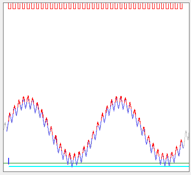
The default parameters simply detect every peak in the selected trace, and because of the noise, there are a lot of peaks! The preview events show as an almost solid bar because there are so many (below left).

Set the Merge foothills threshold to 1, and note that now the noise is merged so that the events reveal the high frequency sine wave (below right: the top trace in the main display).

Complex analysis 1 — Complex hill-valley analysis. The trace contains a mixture of low- and high-frequency sine waves, with added white noise. a. Analysis with the default settings detects numerous hills because each noise peak is a separate hill. b. After merging small foothills with a threshold of 1 (small vertical blue bar), each noise peak is merged with the appropriate peak of the high-frequency sine wave, which is now marked by events.

Complex analysis 2 — Complex hill-valley analysis. The trace contains a mixture of low- and high-frequency sine waves, with added white noise. a. Analysis with the default settings detects numerous hills because each noise peak is a separate hill. b. After merging small foothills with a threshold of 1 (small vertical blue bar), each noise peak is merged with the appropriate peak of the high-frequency sine wave, which is now marked by events.

Now increase the Merge threshold to 4, and note that the fast sine wave peaks are merged to reveal the underlying slow sine wave.

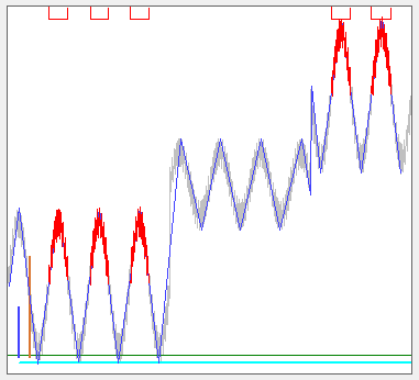
Complex analysis 3 — Complex hill-valley analysis. A Merge threshold of 4 (vertical blue bar) detects the slow sine wave hills.

Now click the Show all toolbar button in the main View.

Note that in the middle section of data, the hills have higher absolute peaks, but smaller peak-to-trough heights than the earlier data (like rolling hills on a high plateau).

Set the Exclude molehills value to 8

Observe that these peaks are no longer marked (below left). The algorithm detects that after merging foothills, the trough-to-peak height of the central hills is below threshold. To be accepted as a peak, both the rising and falling slope heights have to exceed threshold.

Finally, set the Absolute threshold filter to 16
Click Analyse.

Now only the last two high-altitude peaks are detected, because only their peaks reach a value above this threshold (below right).

Complex analysis 4 — Complex hill-valley analysis. a. The central group has been excluded by first merging foothills (threshold 4, vertical blue line) and then excluding molehills (threshold 8, vertical brown line). b. Only the last two hills are above the absolute threshold (16, horizontal green line). Note that merging foothills is essential to detect the low-frequency sine waves, but excluding molehills is no longer necessary.

Complex analysis 5 — Complex hill-valley analysis. a. The central group has been excluded by first merging foothills (threshold 4, vertical blue line) and then excluding molehills (threshold 8, vertical brown line). b. Only the last two hills are above the absolute threshold (16, horizontal green line). Note that merging foothills is essential to detect the low-frequency sine waves, but excluding molehills is no longer necessary.

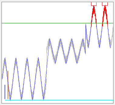
Note that in the latter case the Merge foothills filter is still necessary to detect any of the main peaks, but the Exclude molehills is unnecessary in this case because their peak height is below threshold anyway.

Tutorial Contents

Hill-valley analysis