Burst Detect
Concepts
Subjectively, a burst can be considered to be a consecutive sequence of eventsThe term "event" refers to the digital DataView events, not just "something special that happens in the data". So before you can use this algorithm you need to pre-process the data to detect the occurrences of "something special" and mark them with digital events. such as spikes that are unusually close together. DataView provides two objective methods for detecting such sequences: the “Poisson surprise” method devised by Legendy & Salcman (1985), and the “rank surprise” method of Gourévitch & Eggermont (2007). They both use a statistical method to detect sequences of events which are “surprisingly” close together. The former is based on the parametric Poisson distribution, while the latter is based on the non-parametric rank distribution. DataView also allows manual detection of bursts, where the user decides what constitutes an “unusually close” interval.
In both objective methods in DataView, surprise is defined as –log10(p), where p is the probability of a set of events occurring that close together by chance. Thus a surprise value of 2 reflects a p value of 0.01 (highly significant, in statistical parlance).
In the Poisson method, p is the probability that a number equal to or greater than the actual number of events that occurred within a particular time window, would have occurred within that time window if the spikes had followed a Poisson random distribution with the average frequency of the whole analysis region.
A time window is defined as the time between the first and last event within the analysis region. This is because the amount of "dead space" before the first and after the last event is often aribitrary since it depends on when the recording started and stopped relative to ongoing activity. This means that there is one fewer event contributing to the frequency than the total - the last event does not count. The same is true when calculating the frequency within a burst, e.g. if there are 3 events in a putative burst, the in-burst frequency is 2 divided by the time between the first and third event.
In the rank method, each event interval (on-time to on-time) is labelled with its rank in the total set of intervals, and a burst is then indicated by a contiguous sequence of events whose intervals all have low ranks (i.e. are unusually short). The p value is the probability of finding such a sequence, if in fact the ranks were randomly distributed.
In DataView both objective methods use the “exhaustive surprise maximization” algorithm of Gourévitch & Eggermont. This means that all possible sub-sequences of contiguous events are considered as potential bursts, and the non-overlapping sets with the highest surprise value that exceed the user-set surprise threshold are then accepted as actual bursts. To speed this up and to reduce memory requirements, the total record is broken up into chunks by a user-set maximum in-burst interval. This is NOT used to define bursts themselves, but rather it defines a time value which is definitely the upper limit of what could ever occur within a burst: events which are separated by more than this time interval are definitely either not in a burst at all, or are in separate bursts. Thus the chunks defined by this value can be analysed for bursts independently of one another, which saves on memory. The value does not have to be set precisely, but it is important that it is not set too low, or genuine bursts will be broken into adjacent sub-bursts. You can either set the maximum in-burst interval by visual inspection of the data aided by a histogram display of intervals, or you can set the value as a percentile of the ranked intervals.
The manual method requires the user to set a Maximum start interval (note that this is a completely different concept from the maximum in-burst interval used in the objective methods above). Event intervals are scanned in sequence, and as soon as an interval less than this occurs, it is considered to be at the start of a burst. The burst continues as long as intervals are less than the Maximum continuing in-burst interval, which can be set to be equal to the start interval, or longer. In the latter case, bursts may contain intervals which are longer than those required to start them.
After bursts have been identified, a set of filters can be applied. You can merge bursts which are separated by less than a minimum interval, and you can delete bursts which are below a minimum duration, or which contain less than a minimum number of events.
Examples (simulated)
- Load the file bursts gamma.
This is an event-only file of simulated data (constructed using DataView itself), in which channel a contains brief bursts of high-frequency events superimposed on a lower frequency background. Both types of activity derive from gamma distributions with a shape parameter of 3, and with mean intervals of 25 and 500 ms respectively. Channel b (displaying above channel a) shows the “ground truth” of bursts – its events bracket the high-frequency episodes used in data construction. There are 41 events in channel b (you can check this later), and hence 41 bursts in the data in channel a, although only 9 are visible with the current display viewport. Channel c is a control channel containing a series of events with purely Poisson distribution - there are no "inserted" bursts.
- Select the Event edit: Burst detect menu command to display the Burst Detect dialog box.
This dialog is non-modal, so you can switch away from it to perform other actions if you wish. The default settings tell the program to look for bursts in the Source event channel, which is set at a, and this does indeed contain the bursty data. Any detected bursts will be stored in the Burst event channel, which is set to d (the first empty event channel).
The dialog displays a histogram of inter-event intervals in the source channel. If you move the mouse over the histogram, you can read the X axis values of the cursor location in the box above. By default, the X axis has a logarithmic scale, because this is best for displaying a histogram where the counts decrease as the X-values increase, and it makes the bimodal nature of interval distributions containing bursts clearer. The histogram shows a draggable red cursor, which is linked to the Max in-burst interval parameter. The default value of this parameter is 100 ms, which happens to be appropriate for these data: note that the red cursor is located just to the right of the “valley” which distinguishes between in-burst and out-of-burst intervals.
- Hover over the histogram peaks and note that they occur at about 25 and 500 ms, which fits with the distribution parameters used in data construction (the data are drawn randomly from the distribution, so values will not be exact).
- Uncheck the Log intervals box. The X axis is now linear, and although there is clearly more than one type of interval, the display is much less easy to interpret, so re-check the Log intervals box.
Now we will analyse the bursts. The Poisson surprise method is selected, and the Surprise value is set to 2. These settings are all appropriate, so:
- Click the Analyse button.
Channel d now shows events which almost exactly match those in the ground-truth channel b. Bursts have been successfully detected!
- Activate the Event edit: Event channel properties menu command to activate the Event channel properties dialog.
- Set the Event channel to d.
- Select the Surprise from the Numeric display per event drop-down list.
Note that Surprise is only available on the drop-down list for channel d, because only this channel has been constructed using the Surprise method. - Click OK. The surprise value associated with each burst is now shown on the screen.
Statistics caution: As stated previously, a surprise value of 2 reflects a p value of 0.01, which in normal experimental protocols would be regarded as a "secure" result. However, the burst detection algorithm tests the surprise value repeatedly within a recording, and it is inevitable that in a recording of reasonable length occasional bursts will occur by random chance.
- In the Burst Detect dialog, set the Source channel to c. This has events with a pure Poisson distribution (although with a minimum interval of 2 samples).
- Click Analyse.
Twenty two "bursts" are detected in channel c, of which 6 are visible in the viewport. These each coincide with a period of high event frequency in the source channel, but these are just a natural part of the Poisson distribution.
- Increase the Surprise value to 4. This means that the probability threshold is now 0.0001.
- Click Analyse again.
Now only one "burst" is detected in the Poisson distribution (located outside of the display viewport).
- Reset the Source channel to a, and click Analyse.
With this more demanding probability threshold, 30 of the 41 induced bursts are detected.
The bursts in channel a in these simulated data are extremely obvious. How does the system perform when the situation is less clear?
- Load the file poisson 10 50hz.
This too is simulated data (derived from Neurosim), but the source is more complicated, and, hopefully, a bit more realistic. The bottom trace shows a neuron receiving supra-threshold EPSPs with a Poisson distribution and a mean frequency of 10 Hz. The top trace shows neuron receiving sub-threshold EPSPs, again with a Poisson distribution, but a mean frequency of 50 Hz. In the middle of the record, a pulse of positive current is injected into the top neuron, so that it spikes with each EPSP. There is a synaptic connexion from the top neuron to the bottom neuron, so that there is an increase in spike frequency in the bottom neuron in response. Each spike in the bottom neuron has previously been detected as an event in event channel a, and this is displayed above the lower trace.
- If necessary, select the Event edit: Burst detect menu command to display the Burst Detect dialog box.
The dialog now takes its data from this new file, but the histogram is rather less informative, so this time we will set the maximum interval differently.
- Click the Set button and note that the Max in-burst interval gets set to 431. The In-burst interval %tile is 90%, and this means that 90% of the times between events in the source channel are less than 431 ms. The red cursor in the histogram moves quite far to the right (because only 10% of intervals are above the threshold), but for the surprise methods this is acceptable (see description above).
- Set the burst channel to b (which is currently empty), and make sure that Poisson is selected as the method.
- Click Analyse.
A burst event appears in channel b which almost exactly matches the induced spikes in the upper trace, but remember that the location of this burst is determined programmatically by the timing of the spikes in the lower trace. This (in my opinion) is quite impressive, since visual inspection of the lower trace, without prior knowledge of the upper trace, would not necessarily have led to the conclusion that a burst existed with these timing characteristics.
- Set the method to Rank and the burst channel to c.
- Click Analyse again without changing any other parameters.
A burst is again detected, but it only encompasses the latter part of the Poisson-detected burst. This is consistent with the fact that the Poisson method is tailored to Poisson distributions, which these data more-or-less follow, whereas the rank method is distribution-neutral, but perhaps less effective with actual Poisson data.
- Set the method to Manual and the burst channel to d.
- Click Analyse.
The manual method with these parameters is pretty hopeless, but that is not surprising because we have not set the Maximum start interval to a realistic value.
- Reduce the Bin number of the histogram to 10. Note that the shape of the histogram is very dependent on the chosen bin number, but with 10 bins a bimodal distribution becomes apparent.
- Drag the red cursor to a point on the right side of the valley, so that the Maximum start interval becomes about 60 ms.
- Click Analyse.
At this point your screen should look something like this:
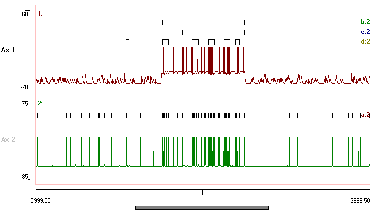
The advantage of the manual method is that it is very much “what you see is what you get” – you have complete control over the rather simple algorithm used to detect bursts, and by combining the manual parameters with post-filtering, it is possible to fine-tune detection to a considerable degree. The Poisson and Rank methods have greater “behind the scenes” intelligence – they use statistical properties within the data to detect bursts that might not be obvious from visual inspection. Whether that is a good thing is a matter for academic judgement.
- Load the file bursts uniform.
- If necessary, , select the Event edit: Burst detect menu command to display the Burst Detect dialog box.
There are very obvious bursts in event channel a, with channel b showing the ground truth used to generate bursts. However, event intervals in this file have a uniform distribution. The background channel a events (i.e. outside of channel b events) have intervals drawn from the range 55 - 500 ms, while the channel a bursts (within channel b events) have intervals drawn from the range 20 - 55 ms. (Details of the data construction are given in comments that can be accessed through the File: Comment menu command.)
- Set the method to Poisson and the burst channel to c.
- Click Analyse.
Some bursts are detected, but most are not.
- Reduce the Surprise value to 1, and click Analyse again.
With this more relaxed criterion, the detected bursts now match the ground truth almost exactly. The poor performance of the Poisson method at the higher surprise value is presumably because the event distribution is not Poisson - thus contravening one of the assumptions underlying the method. However, the distribution-free Rank method does not perform very well either. In fact, it performs less well than the Poisson method with these data, which I find surprising.
Analysis
Once you have detected bursts, it is quite likely that you will want more information about their characteristics. You can use the usual histogram and graphing facilities to display details about the bursts themselves, but you can also drill down into the contents of each burst.
- Re-load the file bursts gamma.
We can use the ground truth event channel b as the marker for bursts, with the events in channel a that occur withinFor one event to be counted as being within an event in another channel, its start time must be greater than or equal to the start time of the enclosing event, and its end time must be less than or equal to the end time of the enclosing event. events in channel b being the burst content.
There are several options for analysis. Here are some.
- Select the Event analyse: List/save event parameters menu command to open the Event Parameter List dialog.
- Check the ID box at the top of the left-hand column.
- Check the Stats (2 in 1) box (about 2/3 down the left column).
- Set Event chan 1 to b (the enclosing channel) and Event chan 2 to a (the events we want to count). I.e. reverse the default channel values.
- Click List.
The Results output lists details of events in channel a that are fully enclosed within events in channel b. There are 41 channel b enclosing events, and so 41 rows of output. The first 3 rows are shown below:
| #ID | On time | Count | Interval avg | Interval S.D. | Dur avg | Dur S.D. |
| 1 | 50 | 9 | 21.6250 | 9.4557 | 1 | 0 |
| 2 | 1340 | 13 | 15.3333 | 8.2609 | 1 | 0 |
| 3 | 2684 | 8 | 28.8571 | 16.6376 | 1 | 0 |
Each row shows the ID of the enclosing event in channel b, the on-time of the enclosing event (this is because we left the On time selection checked in the List dialog), followed by the count of events in channel a fully within that particular event in channel b, the average interval between the enclosed events within that enclosing event, the standard deviation of those intervals, the average duration of the enclosed events, and the standard deviation of those durations. The latter two values are all 1 and 0 respectively, because the channel a events are all point processes.
You can also show a histogram of event count distribution.
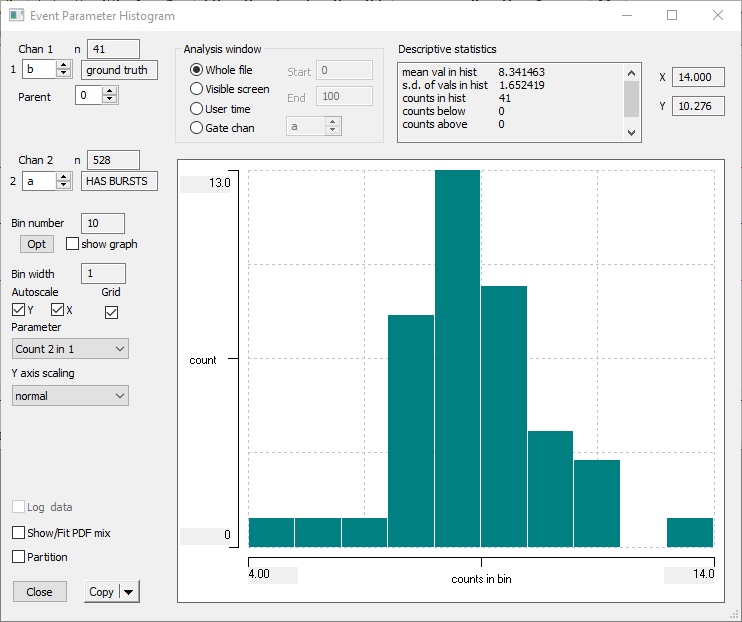
- Select the Histogram/statistics menu command to open the Event Parameter Histogram dialog.
- Select Count 2 in 1 from the Parameter drop-down list.
- Set Chan 1 to b and Chan 2 to a.
You should see a histogram with an approximately Gaussian shape. The modal peak tells you that there are 13 bursts (Y axis) containing 8 events (X axis), and this is the most "popular" burst content. The text box at the top tells you that on average there are ~8.3 events within each burst.