
As we will see in detail in part 7, a serious disadvantage of the Hertzian
dipole is that it suffers from a combination of two problems which can
severely limit is efficiency as an antenna. These are:
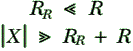
i.e. the value of the radiation resistance is normally much smaller than the
antenna's real resistance, and the antenna's reactance (normally capacitive)
is much larger than the resistance.
For these reasons we find that the Hertzian dipole is not usually a very
efficient antenna at low frequencies. As a result, when we have to use
antennas whose sizes are very small relative to the signal wavelength it can
often make sense to use Magnetic Loop or Ferrite Rod antennas.
Textbooks on antennas or electromagentism often consider a variety of forms
of Magnetic Loop. Some have a circular cross-section, some square. Some have
a length much shorter than their diameter, others are long. Although the
details of these systems vary (for example, their inductance depends on the
ratio of their length to diameter) they are all ‘small’ compared
with the wavelength. As a result we can explain their general behaviour in a
way that ignores many of these details.
When we set up an alternating current in a loop we essentially create a
fluctuating dipole magnet through the center of the loop. The far-field
patterns of the various shapes of loop are all essentially identical as the
dimensions of the loop are ‘too small to be noticed’ from a long
way away since they are all tiny compared with the signal wavelength.
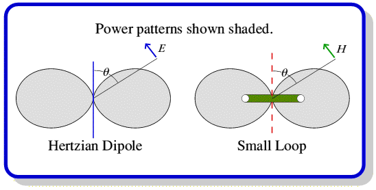
The behaviour of a small loop has some similarities to a Hertzian dipole.
For example, it has the same antenna power pattern, but oriented such
that the nulls – which for a dipole are along the direction of the
dipole wire – are aligned perpendicular to the plane of the loop. The
main difference we’d observe in the far field patterns of that the
electric and magnetic fields have been ‘swapped over’.
Hence, defining the direction angle, theta, to be with respect to the
perpendicular to the loop plane we can say that – for a loop –
the electric field radiated into the ‘far field’ will be
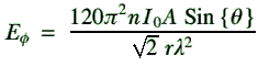
Comparing this with the expression we obtained earlier for a dipole we can
see that it shows the same angular dependence, etc, but is scaled slightly
differently. It also depends upon ratio between the loop’s
cross-sectional area, A, and the wavelength squared rather than the
ratio of the dipole’s length to the wavelength. The other distinction
is that the electric field component is parallel to the plane of the loop
rather than parallel to the dipole wire.
Now if this were all there was to the story, there would be no real
reason to prefer loops to dipoles at low frequencies. However, the loop
turns out (pun?) to have some significant advantages due to the way it
operates. In each case we have defined the radiated field in terms of a peak
current, , on the antenna. As we established in the pervious section it can
be difficult to induce a significant current level onto a dipole. Setting up
a current in a loop is, however, relatively easy. We no longer have the
‘open end’ problem as we can push charge into one end of a
looped wire and draw it out again at the other. Hence we can expect to be
able to obtain relatively high currents (compared to a Hertzian dipole)
quite easily. In addition, we can use a high value for the number of turns,
n, around the loop to multiply up the effect of a given input
current. For these reasons we tend to find that a small loop is easier to
use than a Herzian dipole.
In principle, if a magnetic loop was ‘perfect’ (i.e. it had
perfectly conducting wire) we could expect it to radiate all the power we
drove into the loop. In reality the efficiency of the loop will depend on
the relative levels of the loop’s real (dissipation) resistance and
its radiation resistance. By going through the appropriate calculations we
can find that, for a small loop, the radiation resistance will be

where A is the loop area and lambda is the wavelength.
The metallic resistance of the loop will
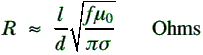
where l is the length of the wire around the loop (i.e. n
times the circumference), d is the diameter of the wire, f is
the signal frequency, and sigma is the conductivity of the metal wires.
In the absence of any resistive losses, the antenna gain of a small loop
(and that of a Hertzian dipole) would be 1·75dB. In reality the
effective gain is reduced by power dissipation in the resistive losses. It
is conventional to describe these losses in terms of a Radiation
Efficiency Factor,
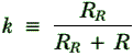
The antenna’s gain (and hence its effective area, etc) are then
degraded by this factor compared to what we’d expect from a
‘perfect’ antenna with the same directional behaviour. In
practice we tend to find that as with the dipole the real resistance tends
to have a higher value than the radiation resistance, hence the loop does
not perform as well as we would wish. Although typical loops have a k
value well below unity they tend to offer higher values than a Hertzian
dipole. Their efficiency can also be dramatically improved by the use of a
Ferrite Rod as will be considered in more detail in part 7.
Summary.
You should now understand that a coherent antenna is a reciprocal device — i.e. that it's behaviour as a transmitter and receiver is the same, but with the ‘video playing the other way’. That it is a form of transformer, which turns one kind of electromagnetic signal into another. You should see how an antenna produces a directional power pattern. That this behaviour can be described in terms of either a Solid Angle, or a Gain, or an Effective Area. You should also know that the way an antenna radiates power can be modelled using a Radiation Resistance. That any resistive losses or reflection can be modelled in terms of a Loss Resistance and an Antenna Reactance, and we have to match the generator/antenna impedances and minimise the loss resistance to get optimum behaviour.


 Content and pages maintained by: Jim Lesurf (jcgl@st-and.ac.uk)
using HTMLEdit3 on a StrongARM powered RISCOS machine.
University of St. Andrews, St Andrews, Fife KY16 9SS, Scotland.