Introduction
This brief webpage briefly describes how to use the Excel add-in "XlXtrFun" to annualise non-annually resolved data-sets. This add-in has been tested on Windows versions of Excel (97-2003).
This is not a tutorial on how to use Excel, so prior knowledge of Excel, add-ins and functions is assumed.
There are two reasons why one might want to do this:
(1) Plot time-series on a common 'Calendar Year' axis. This is simply easier if all time-series have a value for each year.
(2) To facilitate upload of data to the KNMI Explorer for exploratory empirical analysis against climate data. KNMI requires annual values, although be careful about appropriately smoothing your data to account for the original sampling resolution of your data. KNMI allows you to smooth data using a centred moving average, and to overcome aliasing effects, a moving average of roughly 4 times your sampling precision will reduce bias.
e.g.
for 3 year sampling resolution, a 12 year moving average
5 year sampling resolution = 20 year moving average
10 year sampling resolution - 40 year moving average etc etc
NB. The more you smooth, the lower your degrees of freedom will be. This will effect significance greatly.
Download and Installation
The XlXtrFun add-in can be downloaded here. You may have to right click on this link and choose "save target as".
This add-in can do much more than the simple interpolation I describe here. The XlXtrFun Windows Helpfile can be downloaded here. I assume that this file cannot be read on a Macintosh. You may have to right click on this link and choose "save target as".
You now need to move the "XlXtrFun.xll" file to your Office Library folder.
On my computer, the path is: D:\Program Files\Microsoft Office\Office\Library
You can move the helpfile into this folder as well, although it is not needed for the add-in to work.
Now open Excel, click on the Tools menu and click on "Add-Ins" down the menu.
 |
You should now get a dialogue box that lists the available Add-Ins.
 |
Scroll down the list until you see "XlXtrFun " at the bottom. Check the box.
If "XlXtrFun" is not there, you will need to click on the Browse button and look for where you saved/moved the original "XlXtrFun.xll" file.
XlXtrFun should now be installed as a function option in Excel.
Using XlXtrFun to annualise data
The data and results for the following example, can be access here. You may have to right click on this link and choose "save target as".
Firstly, here are some random data, sampled at 5 year resolution, for the last ~120 years. When plotted in Excel, it automatically linearly interpolates between the values, but unfortunately, never provides these 'between-actual-value' interpolations.
 |
Next, you want to create two new columns.
For simplicity's sake, I have named them "year" and "Annual Value"
In the "Year" column, you want to list ALL years from 2000 down to 1880. The easiest way to do this is write in 2000 and 1999, highlight the two cells and then drag on the black square on the bottom right hand corner and drag down until 1880.
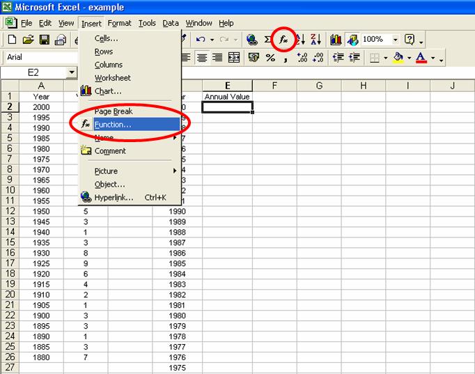
To derive the interpolated values, click on the currently empty 'annual value' cell beside 2000 (E2) and click on insert/past function. Depending on how you have set Excel up, there are two ways to do this. Highlighted in red circles below. If you use Excel regularly, then this is the same process as doing averages, standard deviations, correlations etc etc.
 |
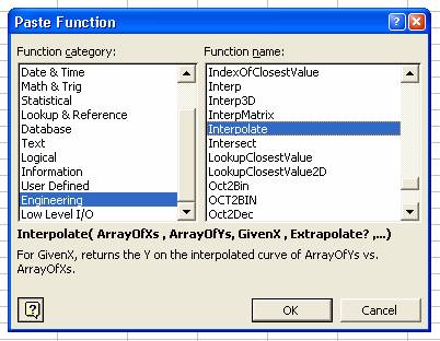
Once you have clicked the insert function button, you will get the "Paste Function" dialogue box.
Scroll down the "Function category" on the left until you come to "Engineering", and then scroll down the "Function name" on the right until you come to "Interpolate". Click OK
 |
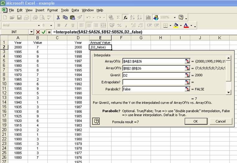
You now need to highlight the relevant field arrays.
Array of Xs - refers to the original "Year" values - i.e. cells A2 to A26. Highlight these cells (A2:A26), but then insert $ symbols to state that this reference array must always stay static - i.e. $A$2:$A$26.
Arrays of Y2 - refers to the original 5 year resolution values. Highlight B2 to B26 in the same way as above for X. Do not forget the $ symbols!!
GivenX = this is the Year value from which the interpolation will be made. For the highlighted cell, you need to click on D2 - in this example.
Important - ensure that you write "false" into the "Parabolic?" field. This will ensure LINEAR interpolation between the values.
Now click on OK and a value of 7 should appear in cell E2. This should be the same value for the year 2000 as in cell B2.
 |
Now all you need to do, is drag the highlight E2 cell (small black square - bottom right hand corner) down the column until you get to year 1880. Depending on your version of Excel, you can also double click on the black square to save time. It should do it automatically.
And voila - you should have values for each year.
 |